Slip Analysis
After specifying the input data, you can now run the slip analysis to calculate the fractures state and other output parameters.
Calculate Slip
The Slip Analysis workflow may be used to analyze the integrity of a fracture or single fault element in Individual Fractures mode or to analyze a set of fractures or fault patches in Set of Fractures mode. The user may switch between these two modes by selecting corresponded Calculation mode.
Individual Fractures In this mode, the algorithm evaluates the stability of each fracture based on the data provided in the Input Definition form. After the calculation is complete, users can select a specific fracture to view its analysis results. To do this, create a Slip Analysis Input View (which is a Well View displaying input logs and fractures as tadpoles) and a Slip Analysis Output View by clicking the Show button in the Analyze Slip section of the popup. Once these views are generated, you can either click on the tadpole symbol representing the fracture of interest in the Slip Analysis Input View or use the slider available in the Slip Analysis Output View to navigate between fractures. In the Slip Analysis Input View, a small red circle around a tadpole in the fracture data track indicates the currently selected fracture. The pole corresponding to this fracture is then displayed in both the Mohr diagram and the stereoplot.
The stresses used to assess fracture stability are derived from the stress input data at the exact depth of the selected fracture. These values - including stress magnitudes, pore pressure, azimuth of SHmax, and Biot coefficient - are calculated through linear interpolation between the nearest data points in the stress input. The interpolated values, along with the fracture’s depth, dip, and dip direction, are listed in the Input Data Table, which can be accessed through the options in the Slip Analysis Output View.
Set of Fractures In this mode the algorithm determines stability for a set of fractures within a specified depth interval. That interval can be specified numerically or graphically. To specify the interval numerically you should select the TVD reference and then specify the TVD of interval midpoint. Window parameter defines the interval range.
Source depth interval can also be defined graphically in the Slip Analysis Input View. Three horizontal red lines appear on the input data tracks to indicate the depth interval. Solid horizontal red line indicates the midpoint of interval, and dashed lines indicates the top and bottom of the interval. The user may modify the depth range and its midpoint interactively.
The stress magnitudes, pore pressure, azimuth of SHmax, and Biot coefficient at the midpoint depth are used to analyze the state of stress on all fractures within the depth window. The values of these parameters are determined by linear interpolation between the nearest stress input data points and are shown in the Input Data Table, which can be accessed through the view options in the Slip Analysis Output View. These reference stresses are used to compute constant stress and pore pressure gradients for the calculation of the shear and normal stress on each fracture plane within the selected interval. The shear and normal stresses calculated at each depth are then normalized by the vertical stress at that depth so that the fracture population within the selected interval can be plotted in a single Mohr diagram. Poles to all analyzed fractures are plotted in the stereoplot. Provided the effective stress ratios are constant throughout the interval over which the analysis is carried out, the results of calculations in Set of Fractures mode are explicitly correct. If not, less than accurate calculations of the shear and normal stress will be displayed. You can adjust the midpoint and interval to redo the calculation.
Data type This option controls the unit system and domain in which the calculated slip-analysis results are displayed. The user can choose between EMW‑XX (Equivalent Mud Weight referenced to the selected TVD reference, where XX reflects the chosen reference such as SS, RT, or GL) and Pressure (absolute pressure values). When EMW‑XX is selected, applicable computed outputs (e.g., Coulomb Failure Function, Critical Pore Pressure and Critical Depletion/Injection) are converted into equivalent mud weight values consistent with the selected TVD reference and are visualized in this normalized domain on both the stereoplot and the Mohr diagram. When Pressure is selected, the same results are presented in absolute pressure units without conversion. This setting affects only the representation and visualization of results; the underlying calculations remain unchanged.
Click (Re)Calculate to start the analysis. The first time you run the analysis, the lock is red, see below for the different colors of the lock and its implication.
|
|
Open When the lock is green and in the open position, the associated algorithm is automatically executed when a change is made to the data’s input. Current status of output data is 'up-to-date'. |
|
|
Locked, No Changes When the lock is blue and in the locked position, the associated algorithm is not updated when a change is made to the data’s input. Current status of output data is 'up-to-date'. |
|
|
Open, Red When the lock is red and in the open position, the associated algorithm is automatically executed when a change is made to the data's input. Current status of output data is 'not-up-to-date', meaning the algorithm was already executed but output data was not calculated/updated due to some errors or lack of input data. |
|
|
Locked, Red When the lock is red and in the locked position, the associated algorithm is not updated when a change is made to the data's input. Current status of output data is 'not-up-to-date'. To apply the updates, you need to click the associated (Re)Calculation button. |
Analyze Slip
Once calculation completed, the user may select which sets of fractures to display in the Slip Analysis Input View and Slip Analysis Output View by checking or unchecking the Visibility boxes in the analysis results table. This may be useful when there are thousands of fractures in the input data set. For example, by unchecking all but the critically stressed fractures, application will display only the critically stressed fractures in all views.
The analysis results table also provides a summary of the number of fractures categorized by their stability state: critically stressed, not critically stressed, and not analyzed. In addition to this quantitative overview, the table also explains the meaning of the fracture icons used for visualization in both the Slip Analysis Input View and the Slip Analysis Output View. These icons help users quickly identify the status and characteristics of each fracture within the analysis workflow.

|
Critically stressed fractures (white - for stereoplot, red - for all other plots) |

|
Critically stressed S3-normal fractures (white outlined - for stereoplot, red outlined - for all other plots). |

|
Not critically stressed fractures |

|
Not critically stressed S3-normal fractures. |

|
Fractures not analyzed. |
Using Tadpoles color option the user can choose between two display options for tadpoles visualization in the Slip Analysis Input View: Fixed and Variable. The Fixed option displays tadpoles in red and black (with green inside for S-3 normal fractures), as described above. The Variable option allows tadpoles to be color-coded based on the calculated values of a selected output parameter, such as Coulomb Failure Function, Critical Pore Pressure, Critical Depletion/Injection, or Critical Friction.
It is important to note that the tadpole plot uses the same color palette as the one shown in the Slip Analysis Output View below the stereoplot but applies its own color scale values. These values typically differ from those used in the stereoplot because the tadpole plot uses the minimum and maximum from output values calculated for each fracture. In contrast, the stereoplot uses the minimum and maximum from plot data, which is calculated for each degree of Dip and Dip Azimuth.
Click Show to open a Slip Analysis Input View and Slip Analysis Output View and see the calculation results.
Using Slip Analysis Results to Plan a Drilling Trajectory
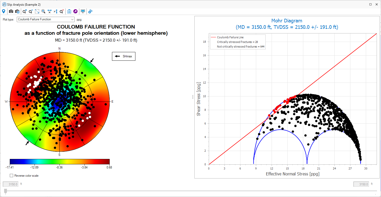
Figure MF2. Slip Analysis results. click to enlarge
The analysis result shown in picture above reveals that within the region of interest, there are critically stressed fractures dipping steeply to the southeast and to the northwest. An optimal trajectory for this well that minimizes the risk of fluid losses while drilling would be parallel to the critically stressed features. On the other hand, an optimal trajectory to maximize reservoir permeability for this well would be perpendicular to critically stressed faults.
If the fracture population appears to have a predominant preferred orientation, then the most productive well will be the one that is drilled into the highest concentration of critically stressed (white) fractures. In this case, there are a slightly greater number of fractures with poles to the NW than there are with poles to the NE, so the optimal trajectory for a productive well would be at a deviation of approximately 60° at an azimuth of N45°W.