Elasticity Around The Hole View

The example of the view shown below is created using temperature effects. It shows the wellbore cross section on the left-hand side. Displayed is the uniaxial rock strength, UCS, required to prevent breakout initiation. Colorless (gray) regions indicate areas of negative effective stress where tensile failure is expected. On the right-hand side there is a plot showing thermal stresses as a function of normalized radial distance (distance/borehole radius) from the borehole. You can change the left-hand plot interactively to display the required rock strength, the stress trajectories in a plane perpendicular to the hole (Stress crosses), or any stress component by selecting it from the Plot type drop-down list. When you select a new option, the view is updated immediately.

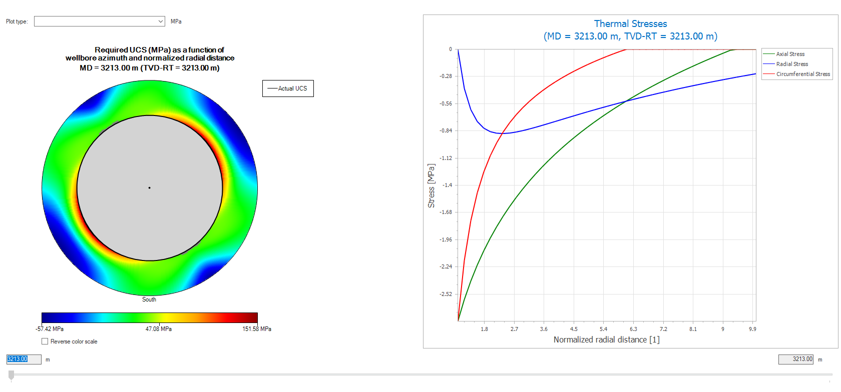
Example of the Elasticity Around The Hole View, with only thermal effects selected.    click to enlarge

You can click outside the wellbore cross section, or click inside the wellbore cross section, to open a new window, called Profile View, displaying the selected parameter as a function of radius or azimuth. You can change the Profile View by clicking and dragging the white line in the Around The Hole View to a new location, see video to understand this behavior.

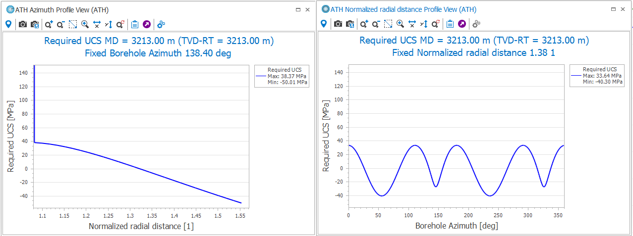
Example of the two Profile Views    click to enlarge

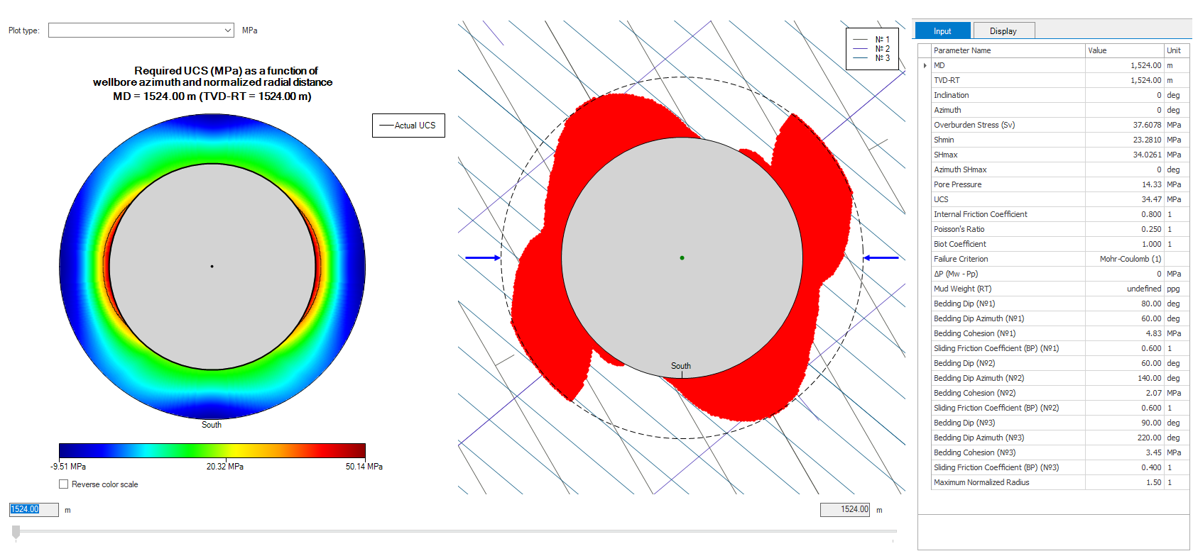
The example of the view shown below, is created using the bedding planes option on the Advanced Mode form, and selecting one plane of weakness on the Around the Hole form. It shows the wellbore cross section on the left-hand side, where you can display any of the Effective stress components by selecting the desired parameter from the Plot type drop-down list.

On the right-hand side, the view shows a cross-sectional view of the borehole looking down its axis. Zones within which the stress exceeds the limits beyond which failure will occur, are colored in red. Parallel lines show the orientations of the anisotropic weak planes projected into the plane perpendicular to the wellbore axis. Blue arrows indicate the direction of maximum compression projected onto the borehole cross section. The ears on both sides result from failure due to strength anisotropy of the rock. When failure is restricted to the extreme near-wellbore wall region, red dots indicate its extent. The zone of failure at the center of each failure region is delineated in this manner. The outlined failure zones are not symmetric with respect to the foliation orientation, because the stress and weak planes do not share a plane of symmetry. In this view, the Extract profile is not possible, because there are only two states – either there is failure, or there isn‘t.

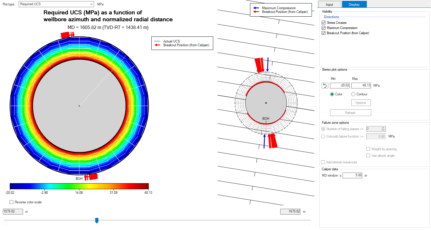
Example of the Elasticity Around The Hole View showing the direction of maximum compression along with breakout position from the caliper log analysis, with bedding planes selected, and one plane of weakness.    click to enlarge

You can click outside the wellbore cross section, or click inside the wellbore cross section, to open a new window, called Profile View, displaying the selected parameter as a function of radius or azimuth. You can change the Profile View by clicking and dragging the white line in the Around The Hole View to a new location, see link to video.

The example of the view shown below, is created using the bedding planes option on the Advanced Mode form, and selecting orthotropic strength on the Around the Hole form. It shows the wellbore cross section on the left-hand side, where you can display any of the Effective stress components by selecting the desired parameter from the Plot type drop-down list.

On the right-hand side, the view shows a cross-sectional view of the borehole looking down its axis. Zones within which the stress exceeds the limits beyond which failure will occur, are colored in red. Note that the shape of the zone of failure of an orthotropic rock is distinctly different from that of a rock with strength anisotropy, characterized by intrinsically weak planes such as foliation or bedding surfaces, like the example listed above (one plane of weakness). Failure of a material with orthotropic rock strength is similar to failure of an isotropic material, and is controlled by the isotropic strength parameters as well as the amount of anisotropy determined by the values of A and B.

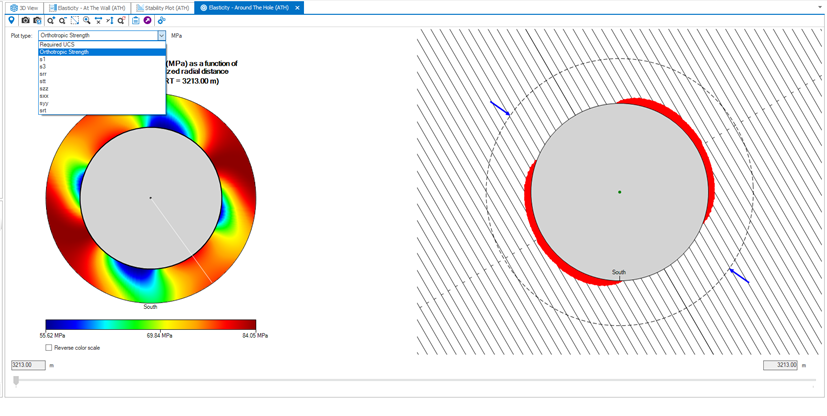
Example of the Elasticity Around The Hole View, with bedding planes selected, and orthotropic strength.    click to enlarge

You can click outside the wellbore cross section, or click inside the wellbore cross section, to open a new window, called Profile View, displaying the selected parameter as a function of radius or azimuth. You can change the Profile View by clicking and dragging the white line in the Around The Hole View to a new location, see link to video.

The example of the view shown below, is created using the bedding planes option on the Advanced Mode form, and selecting multiple planes of weakness on the Around the Hole form. It shows the wellbore cross section on the left-hand side, where you can display any of the Effective stress components by selecting the desired parameter from the Plot type drop-down list.

On the right-hand side, the view shows a cross-sectional view of the borehole looking down its axis. It shows the output result of running the multiple fractures analysis, which shows the well in cross section together with a zone of failure (red color) and the individual fracture sets as they would appear if they were cut by a plane perpendicular to the hole axis.

Each fracture set is displayed in a different color. In this case, the first family set is in black, the second set is electric blue, and the third family is light blue. The distance between the lines corresponds to the real distance between fractures in the borehole cross section (which depends on the fracture spacing and the angle between the well axis and the fracture). Short tick marks indicate the fracture dip direction. Thus, fractures parallel to the hole appear at distances equal to the input spacing and with no tic mark, and fractures perpendicular to the hole do not appear at all, as they lie in the plane of the image. Each fracture set is represented by a line through the center of the well, with additional lines at the appropriate spacings on each side. By default, the zone within which any of the multiple fracture sets is predicted to slip, is colored in red.

Example of the Elasticity Around The Hole View, with bedding planes selected, and multiple planes of weakness.    click to enlarge

The zone of failure can be defined either in terms of the number of planes for which failure would occur, or in terms of a cumulative measure of the coulomb failure criterion (CFF). The default mode is the number of failing planes. To switch between the default display and the alternative of using the coulomb failure function, use the appropriate radio button available in the Display tab in the Settings section. If this section is not visible in your view, click the options icon in the toolbar to show it. To add the zone of failure due to intrinsic breakouts that occur when the stresses exceed the strength of the intact rock, select the Add intrinsic breakouts checkbox beneath the pair of radio buttons. To hide the intrinsic breakouts, uncheck the box. For more details, see Display settings for the zone of failure.

While using the MW to Trigger Slip tool (Borehole Stress > ATH Tools) to determine the critical MW that triggers the shear slip in fractures, the results are shown on the Elasticity Around The Hole View. On the view, the Plot type is selected as Mud Weight to trigger slip. If your Model Definition is using the Log based calculation mode, then a Measured Depth (MD) slider is available at the bottom that you use to modify to plot results for specified depth. If the calculation mode is Depth based then the results plotted for the specified MD.

Use the Elasticity view toolbar to change the plot display or export the plot or data using clipboard options. Use the Options button to view the input parameters and also change visibility or plot contouring.

The example in the plot below show the critical mud weight to trigger slip, with constant MW, as a function of wellbore azimuth and normalized radial distance. You can also activate the Profile Views to understand the relationship with borehole azimuth or the normalized radial distance. The profile views also consists of the Elasticity view toolbar for exporting and visualizing the data. For the profile views, the white line from the center of the borehole to the maximum normalized radius, or the white circle between the borehole and the circle defined by maximum normalized radius, sets the reference for the plotted data. You can drag the white line or the white circle to change the reference and the plots are updated interactively. This behavior is displayed properly in the video below.

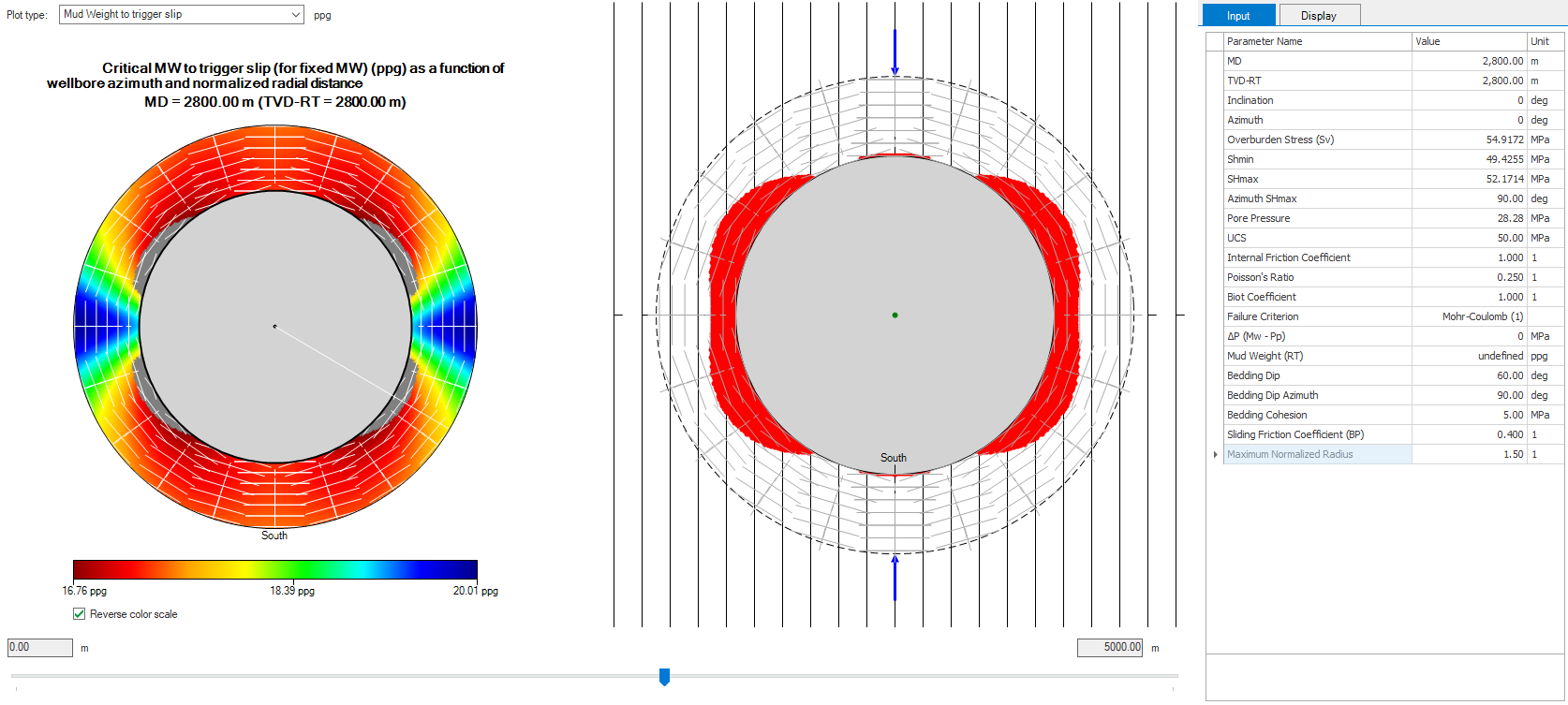
Example of the Elasticity Around The Hole View, displaying the plot for the MW to Trigger Slip, using Log based calculation method and single plane of weakness.    click to enlarge

You can click outside the wellbore cross section, or click inside the wellbore cross section, to open a new window, called Profile View, displaying the selected parameter as a function of radius or azimuth. You can change the Profile View by clicking and dragging the white line in the Around The Hole View to a new location, see the video below.