Slip Analysis Output View
The results of the Slip Analysis workflow are presented in a single, comprehensive output view. Additionally, separate histogram views for selected output parameters can be generated (see MohrFracs Histograms for details). Input data as a function of depth are displayed in the Slip Analysis Input View, which consists of a well view with two tracks: one for stress data and another for fracture data from the Input Definition form.
Fracture orientations are visualized using tadpole symbols plotted by depth. The horizontal position of each tadpole indicates the fracture dip, while the direction of the line extending from the point represents the dip direction, with north oriented at the top of the plot. Tadpoles outside the analysis range are shown in gray. Green tadpoles represent fracture planes approximately perpendicular to the least principal stress (S3-normal fractures). By default, critically stressed fractures are shown in red, and non-critically stressed fractures in black. If a fracture is S3-normal, its tadpole is outlined in red or black, corresponding to its stress state. Users also have the option to color tadpoles based on calculated values of selected output parameters, such as CFF, Critical Pore Pressure, Critical Depletion/Injection, or Critical Friction (see Slip Analysis for details).
The results of a Slip Analysis are displayed graphically in two plots within the Slip Analysis Output View.
Stereoplot
The left plot is a stereoplot showing a lower hemisphere projection of fracture pole orientations, with each pole representing the orientation of a fracture plane.
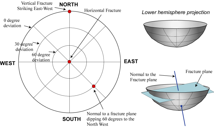
Figure MF3. Fracture planes are represented by the pole to the plane on lower hemisphere projection orientations. click to enlarge
By default, the color at each point in the stereoplot represents the magnitude of the Coulomb Failure Function for a fracture with the corresponding dip and dip direction. The Coulomb Failure Function (CFF) is defined as
CFF = Tau - μ * (Sn - Pp)
where Tau and Sn are the shear and normal stress acting on a fracture, Pp is the pore pressure, and μ is the coefficient of sliding friction. In general, "cool" colors (blues) indicate relatively stable fracture orientations (more negative CFF) and "warm" colors (orange–red) indicate less stable fracture orientations (more positive CFF). Poles to critically stressed fractures (CFF > 0) are shown in the lower hemisphere projection as white. Poles to non-critically stressed fractures (CFF < 0) are colored black. Fractures that are S3-normal are colored green surrounded with white or black depending on whether or not they are also critically stressed. Arrows on the outside of the stereoplot indicate the direction of the maximum horizontal stress.
In addition to the default display of Coulomb failure function (CFF), stereoplot can display the critical pore pressure, critical depletion or injection, or critical friction coefficient in the lower or upper hemisphere projection. Slip Analysis algorithm calculates these values by determining the conditions required for the Coulomb failure function to be equal to zero (CFF = 0). To select the desired output parameter, use the Plot type drop-down.
Mohr Diagram
The lower plot on the right side of the analysis window is a Mohr diagram. Stress states on fracture planes are displayed on the diagram according to the magnitudes of the shear and effective normal stresses acting on the plane. Critically stressed fracture planes, which plot above the red Mohr-Coulomb failure line, are shown in red. The slope of the failure line is equal to the coefficient of sliding friction (μ). MohrFracs module defaults to a zero cohesion. This is normally reasonable because while cohesion of fracture surfaces is finite, it is generally orders of magnitude smaller than the principal stresses. The user has the option to define a non-zero cohesion in the Input Definition form. A finite cohesion affects the Mohr-Coulomb line in the Mohr diagram. Under the Mohr Diagram, the analysis window displays numbers N of critically stressed fractures, non-critically stressed fractures, and non-analyzed fractures.
Output View toolbar

|
Probe tool When activated, hover over the data in the stereoplot or Mohr diagram to display the property data. |

|
Copy view to clipboard Copy the current view to the clipboard for use in other applications. |

|
Save view to file Save the current view to a file with a name and location you specify. |

|
Zoom in Incrementally zoom in on the Mohr diagram. |

|
Zoom out Incrementally zoom out on the Mohr diagram. |
|
|
Zoom rectangle Turns the cursor into a zooming tool. When this option is active, click and drag a box inside the Mohr diagram around the data you want to view in better detail. |
|
|
Zoom on both axes Incrementally zooms in equally along both axes of Mohr diagram. |
|
|
Zoom on the horizontal axis Zooms the Mohr diagram only along the horizontal direction. |
|
|
Zoom on the vertical axis Zooms the Mohr diagram only along the vertical direction. |
|
|
Reset zoom Clear all zoom changes in the Mohr diagram. |
|
|
Export to Clipboard Copies the numerical stereoplot data to the clipboard, allowing it to be pasted into external applications. |

|
Export to File Exports the numerical stereoplot data to a *.txt. file. |
|
|
Options Shows all the view options. |
View Options
Input
This tab displays a table containing all values used in the calculation. In Individual Fractures mode, the values shown correspond to the input data at the depth of the currently selected fracture. In Set of Fractures mode, the values represent data at the midpoint depth of the defined interval. In this mode, dip and dip azimuth values are not displayed, as multiple fractures are visualized simultaneously in the plots and individual orientation data is not applicable.
Display
This tab provides options for customizing how data is visualized in the plots.
Plot options Specify color scale limits and contouring options for the stereoplot .
Min Minimum values for the stereoplot color scale. All values smaller than minimum will be excluded from visualization in the plot.
Max Maximum value for the stereoplot color scale. All values greater than maximum will be rendered using color of maximum value.
Min and Max can be reset to original values using the Reset button ![]()
Color Select this option to render the stereoplot using Color Mode.
Contour Select this option to render the stereoplot using Contour Mode. Contouring settings can be customized through a separate dialog, which is accessible by clicking the Options button.
Lower Hemisphere Select this option to render stereoplot using Lower Hemisphere projection.
Upper Hemisphere Select this option to render stereoplot using Upper Hemisphere projection.
Show slip When this option is enabled, stereoplot displays the plane of the fracture and a tadpole showing slip direction.
Refresh If any of the display parameters are changed, you must press this button to update the plots rendering.