Stress Polygon view
The Stress Polygon view displays the results of a completed UCS or Breakout profile calculation executed on the UCS / BO Profiles form. Present in every Stress Polygon view is a polygon outlined in black that defines the limits of Mohr-Coulomb failure for frictional equilibrium of pre-existing faults. These limits are independent of anything related to the wellbore and depends only on the pore pressure, the vertical stress, and the value of sliding friction. Plotted with the polygon are the magnitudes of the horizontal stresses consistent with failure occurrences as a function of compressive (red contours) and tensile (blue contours) strength of the rock. The stress state must be inside of this polygon because the strength of the crust does not allow a larger stress difference between the greatest and least principal stresses. Normal faulting, strike-slip faulting and reverse faulting stress conditions are all separated in the view by dashed lines.
When a BO profile is chosen, the stress polygon view plots contours of breakout widths that would occur for the defined rock strength and the horizontal stress magnitudes.
The toolbar at the top of the Stress Polygon View contains a set of tools to customize the view and make it easier for you to inspect your data.

|
Probe tool When activated, hover over the data in the view to display the object and property data. |

|
Copy view to clipboard Copy the current view to the clipboard for use in other applications. |

|
Save view to file Save the current view to a file with a name and location you specify. |

|
Zoom in Incrementally zoom in on the view. |

|
Zoom out Incrementally zoom out on the view. |
|
|
Zoom rectangle Turns the cursor into a zooming tool. When this option is active, click and drag a box around the data you want to view in better detail. |
|
|
Zoom on both axes Incrementally zooms in equally along both axes. |
|
|
Zoom on the horizontal axis Zooms the view only along the horizontal direction. |
|
|
Zoom on the vertical axis Zooms the view only along the vertical direction. |
|
|
Reset zoom Clear all zoom changes. |
|
|
Export to Clipboard Copies the numerical plot data to the clipboard, allowing it to be pasted into external applications. |
|
|
Export to File Exports the numerical plot data to a *.txt. file. |

|
Create calibration points Pick a calibration point in the stress polygon to show SHmax and Shmin which are saved as log properties appended with the case name. |
|
|
Options Shows the input data used in the calculations and all the display options. |
Clicking on the Options icon ![]() in the view toolbar opens the options pane with multiple tabs:
in the view toolbar opens the options pane with multiple tabs:
Input In this tab, you can view the input parameters and the assigned values.
Contours Here you can add contours of the inclination with respect to the wellbore axis along which drilling-induced tensile fractures are likely to form. Select a stress profile from the drop down menu and the Min, Max and Increment values are populated for the selected option.
Display In this tab, you can check or uncheck the stresses that are plotted on the view.
Constrains In this tab, you can set various constrains to visualize and compare the stress states.
Shading settings Create a shaded polygon by entering the Min and Max values for stress profiles on the plot. Provide the Min and Max values for Shmin. Check the checkbox adjacent to UCS and/or T0 to activate the fields, and enter the respective Min and Max values. Click Apply to display the transparent shaded regions are created within the stress polygon based on the values entered in the fields. By default, shaded area for UCS is shown in red while the shaded area for T0 is shown in blue. Check the checkbox adjacent to Compare to add the shaded region in the underlying Shading comparison sub-section. You can add shaded areas at different depths for the active 1D case and also from another case within the same solution. Note that the shaded areas are displayed only if the values fall within the stress envelope.
Shading comparison This section tabulates the shaded areas that have been added for comparison. You can check or uncheck the checkbox in the Use column to show or hide the shaded area. The second and third column shows the associated 'Case' name and the corresponding 'Measured Depth' value, respectively. In the last column you can change the color of the shaded area boundary. Click on the Compare button to show the checked cases in comparison with the primary shaded region that you entered in the 'Shading settings'. Click the Compare button again to hide the comparison. Check the checkbox adjacent to 'Convert to current depth' to convert the compared areas to the current depth displayed on the plot. Note that the compare functionality is only applicable for 'Log based' calculation modes.
Logs Use the checkboxes to activate the 'Show Shmin' and 'Show SHmax' fields, and select the stress logs from the drop down menu that you want to display on the plot.
Intercepting SHmax In this sub-section, you can interpolate the value for SHmax by providing an input for Shmin along with the values for UCS and/or T0. The corresponding intercepted SHmax value on the plot is shown in the adjacent fields. On the plot, you can see the intercepted values with a dotted line for UCS and T0. By default, the interception for UCS is shown with a dotted red line and for T0 is shown with a dotted blue line.
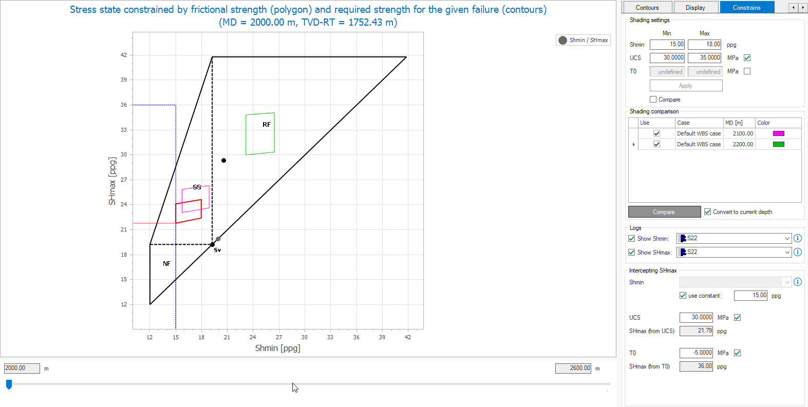
The Stress Polygon View showing the comparison between shaded areas that were added in the Shading comparison section. Note that the compared areas have been converted to the current depth in the example (i.e., 2000 m MD).The Options pane on the right side also shows the selected stress logs for Shmin and SHmax along with the interception points for SHmax. click to enlarge