Interpreting seismic data
Once you have imported seismic trace data in your model, you can start interpreting faults, horizons, unconformities or any other geological event from your seismic survey. You can do this either manually by creating polylines in your 3D View or Seismic View, or (semi) automatically using autotracking functionality of the Editing Tools. The Editing Tools are accessible via Workspace > Tools > Editing Tools. It depends on the view you are in, whether you have 2D or 3D seismic tools available.
Most of the time you will interpret seismic data on standard seismic sections (Inlines, Crosslines, Depth/Time slices) that you visualize in the Seismic View or 3D View. You can also use the functionality described hereafter for seismic data displayed on cross sections.
Creating a seismic interpretation
Before using the seismic interpretation tools, you must have created a Seismic Interpretation folder in the JewelExplorer. If you have not created a Seismic Interpretation folder yet, go to prepare > Seismic > Create Interpretation (when the Assign Data form opens automatically during this process, click OK without assigning any surfaces, since you want to start a seismic interpretation from scratch). Once the folder for this new Seismic Interpretation is created in the JewelExplorer, you are ready to add horizon, fault, intrusion and unconformity interpretations to this folder.
![]() Creating and interpreting a horizon, unconformity or intrusion in the Seismic View or 3D View
Creating and interpreting a horizon, unconformity or intrusion in the Seismic View or 3D View
Activate (click on) the Seismic Interpretation in the JewelExplorer to which you want to add the horizon, intrusion or unconformity. Then go to Workspace > Tools > Editing Tools: the floating palette opens.
The Create New Horizon ![]() , Create New Fault
, Create New Fault  , Create New Intrusion
  and Create New Unconformity
 ![]() icons become available in the floating palette. Click on the icon of your choice, and a new horizon, intrusion or unconformity (with a 2D grid representation) is created in the relevant folder under the Seismic Interpretation in the JewelExplorer.
icons become available in the floating palette. Click on the icon of your choice, and a new horizon, intrusion or unconformity (with a 2D grid representation) is created in the relevant folder under the Seismic Interpretation in the JewelExplorer.
The new 2D grid:
- Will automatically receive the resolution of the Seismic Interpretation.
- Will retain its resolution during interpretation, even when the resolution of the seismic volume is different (for example when the resolution of the seismic volume is coarser than the resolution of the 2D grid, the auto-tracking tool will fill in the lattice of the 2D grid with undefined values).
Activate the newly created event and go to Workspace > Tools > Editing tools to open the floating palette. On the palette, the 2D and 3D autotracking tools  are available.
![]() 2D Manual Tracking (Shortcut key: M) A single click on the seismic slice creates a seed, a straight line of nodes is generated between this point and the next clicked location.
2D Manual Tracking (Shortcut key: M) A single click on the seismic slice creates a seed, a straight line of nodes is generated between this point and the next clicked location.
![]() 2D Single Autotracking (Shortcut key: S) A single click on the seismic slice creates a seed, and a line is generated from this seed.
2D Single Autotracking (Shortcut key: S) A single click on the seismic slice creates a seed, and a line is generated from this seed.
![]() 2D Two Point Autotracking (Shortcut key: T) This mode requires two seed points. First you have to click the start seed point on the seismic slice. Nothing will happen until the second seed point is clicked. Now the tracking will operate from the initial seed to the second seed. In this manner, more control can be given over the resulting tracked lines
2D Two Point Autotracking (Shortcut key: T) This mode requires two seed points. First you have to click the start seed point on the seismic slice. Nothing will happen until the second seed point is clicked. Now the tracking will operate from the initial seed to the second seed. In this manner, more control can be given over the resulting tracked lines
![]() 2D Continuous Autotracking (Shortcut key: Ctrl+T) This mode works similar to two point autotracking. Here the second seed point of a tracking operation will be the first seed point of the next tracking operation. This can save a lot of mouse clicks when continuous lines are desired.
2D Continuous Autotracking (Shortcut key: Ctrl+T) This mode works similar to two point autotracking. Here the second seed point of a tracking operation will be the first seed point of the next tracking operation. This can save a lot of mouse clicks when continuous lines are desired.
![]() 3D Autotracking (Shortcut key: A) Autotracking works automatically in all directions. Dependent on the object you are interpreting, the result of the 3D autotracking consists of polylines or a 2D grid, stored in the 'Horizons', 'Intrusions' or 'Unconformities' folder in the JewelExplorer.
3D Autotracking (Shortcut key: A) Autotracking works automatically in all directions. Dependent on the object you are interpreting, the result of the 3D autotracking consists of polylines or a 2D grid, stored in the 'Horizons', 'Intrusions' or 'Unconformities' folder in the JewelExplorer.
 Remove Nodes Under Line (Shortcut key: Ctrl+L) Draw a line on a 2D grid and remove all the nodes under this line. Select the 2D grid and then select the tool. In your 3D view, click to mark the beginning of the line, move your mouse to the desired end point of the line and click to finish the line. All nodes under the line will be deleted.
 Remove Node (Shortcut key: Ctrl+Q) Remove the selected node(s) from the 2D grid. A single click on the seismic slice starts the selection, a second click finishes the selection. All nodes in between will be deleted.
Settings for autotracking tools
The seismic autotracking tools require specific autotrack settings. You specify these in the settings section on the floating palette, which automatically shows when clicking on one of the tools:
- Pick Type Choose your pick position from the following options:
- Peak: Searches for a maximum value by fitting a quadratic function through sample points to calculate the exact depth value and property value of the maximum.
- Trough: Searches for a minimum value by fitting a quadratic function through sample points to calculate the exact depth value and property value of the minimum.
- Crossing at value, ascending: Searches for the wiggle trace or property curve value that is entered in the Crossing value entry box. When the crossing value is 0, this is where the wiggle trace is moving from negative to positive polarity with increasing depth. Or, when you have entered another value, where the property curve is moving from a lower to a higher value with increasing depth, passing the value you have entered.
- Crossing at value, descending: Searches for the wiggle trace or property curve value that is entered in the Crossing value entry box. When the crossing value is 0, this is where the wiggle trace is moving from positive to negative polarity with increasing depth. Or, when you have entered another value, where the property curve is moving from a higher to a lower value with increasing depth, passing the value you have entered.
- Crossing value (only active when a 'Crossing at value' option is selected) Enter a value to use with the 'Crossing at value' option. By default, the value is set to 0. When interpreting seismic trace data, do not change this value.
- Tolerance Enter the tolerance (+/-), which is the threshold for amplitude similarity. A value similarity set to (for example) 10%, allows seismic autotracking to diverge 10% around the reference value.
- Vertical constraint Set this value to the maximal vertical distance that you allow the autotracked data points to span from it's shallowest to its deepest point. This functionality overrules the value similarity, which means that even when autotrack settings with respect to the value similarity are met (see previous section), the autotrack will end if the vertical limit is reached.
- Horizontal constraint This value represents the maximum number of bins which will be autotracked around your pick position. For the bin size ('resolution'), see the Property Inspector > Seismic Survey section.
- Sampling increment This value determines the sample point increment used for autotracking. A value of 1 means every segment (inline/crossline) will be used for autotracking.
- Stop at discontinuity Check the 'Stop at discontinuity' check box if you want autotracking to stop when encountering a fault (choose a model from the Model drop-down list). Discontinuity awareness is only effective within the depth range you specify in the Start TVDSS and End TVDSS. By default, the depth values are set from the top to base of your model, causing autotracking to stop at any fault in your model (irrespective of its depth). Note that the fault needs to be a tri-mesh to be taken into account, and that the selected model has the same resolution as the currently interpreted surface.
- Seed sampling / Trace sampling Seed sampling will autotrack values using the initially clicked sample point as reference value; Trace sampling will autotrack values using the last tracked data point as reference value.
- Overwrite existing picks If a track of data points already exist, checking this box during autotracking will ignore the existing data points and overwrite with a new track. If the box is not checked, the autotrack will stop if an existing track is encountered.
- Lock selected object Check this box to lock the surface while interpreting. This prevents automatic switching to another object in case you click on an interpretation line of another surface.
Advanced settings
When you are working with the seismic editing tools, it might be helpful to change the display filter of your seismic volume from Cubic B-Spline to No Interpolation.
![]() Creating and interpreting a fault in the Seismic View or 3D View
Creating and interpreting a fault in the Seismic View or 3D View
Activate (click on) the Seismic Interpretation in the JewelExplorer to which you want to add the fault. Then go Workspace > Tools > Editing Tools: the floating palette opens.
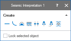
Create tools for a seismic interpretation click to enlarge
Click on the Create new fault icon ; a new fault (with a polyline set representation) is created in the Faults folder of the Seismic Interpretation in the JewelExplorer.
Activate this new polyline set and go to Workspace > Tools > Editing Tools to open the floating palette. The floating palette now shows the polyline set tools, which you can use to interpret the fault. The first icon to use is most probably Add Polyline, since your polyline set is still empty and does not contain polylines yet. Once the polyline set contains polylines, the other icons can be used as well (see Graphically editing polylines).
When you have interpreted a significant amount of polylines for your new fault and you want to review your results in the 3D View, you can triangulate these polylines using the Triangulation Settings form (prepare > Seismic).