Clay content calculation methods

On the Fault Clay Content form (model > Fault Seal > Fault Seal Modeling > Fault Clay Content) three methods are available to calculate clay content in the fault zone:

Shale Gouge Ratio (SGR), after Yielding et al. (1997).
Shale Smear Factor (SSF), after Lindsay et al. (1993) and Yielding et al. (1997).
A combination of the two.

Each clay content method creates its own set of properties which will be added to the 'Fault Seal' surface set in the JewelExplorer. See below for a detailed explanation per method, including a calculation example and an overview of the properties generated in the JewelExplorer.

3D Grid input

For all three the methods, input to the calculations is as follows:

Input to the clay content calculations comes from the grid cell properties of the cells located directly next to the fault, i.e. the cells cut by the fault.
At each calculation point, the input to that calculation is derived from the fault slipped sequence. The slipped sequence is the sequence of layers (more specifically, the grid cells) that have passed the point of calculation on the fault plane. Note that even when a small proportion of a grid cell slipped past a point of calculation, that cell is considered part of the slipped sequence (partially slipped grid cells are not handled explicitly) and as such input to the calculation.

Method 1 - Clay mixing 'Shale Gouge Ratio' (SGR)

This method is an estimation of the proportion of shale in the fault zone that implicitly assumes that fault rock represents an evenly mixed aggregate of the faulted reservoir sequence. It is calculated as a simple arithmetic average (layer thickness weighted average) of the Vshale of all layers of the slipped sequence. This method produces a gradually changing clay value along the fault. SGR outcomes range from 0 to 1.

Formula

where:

V_cl =V_sh of the layer

ΔZi = Layer thickness

Calculation example

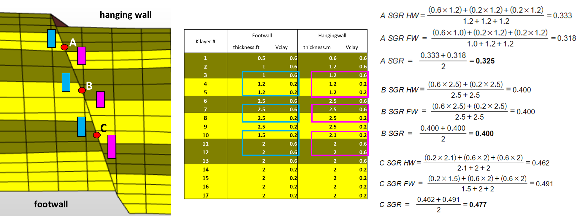
In this example SGR is calculated for point A, B and C (left image). For each of these points, the slipped sequence is determined in the hanging wall and in the footwall (indicated in blue and pink, left image). As a general rule, only layer properties of layers within the slipped sequence are input to the calculation, which is performed separately for the hanging wall and footwall. The boxes in the middle image indicate which layers (with their respective SGR values) are included in the SGR calculation of point A (upper two boxes), point B (middle two boxes) and point C (lower two boxes). These values are combined as shown in the formulas on the right, where you see 'HW' and 'FW' per point of calculation, as well as the average. All three these outcomes are generated as properties in the JewelExplorer, called SGR hanging wall, SGR footwall and SGR average.

Generated properties

Three properties are generated:

SGR average: Average of the SGR hanging wall and SGR footwall of the slipped sequence at the point of calculation (e.g. calculation example 'A SGR' in the image above).

SGR hanging wall: The (layer thickness) weighted average of Vshale of the hanging wall layers of the slipped sequence at the point of calculation (e.g. calculation example 'A SGR HW' in the image above).

SGR footwall: The (layer thickness) weighted average of Vshale of the footwall layers of the slipped sequence at the point of calculation (e.g. calculation example 'A SGR FW' in the image above).

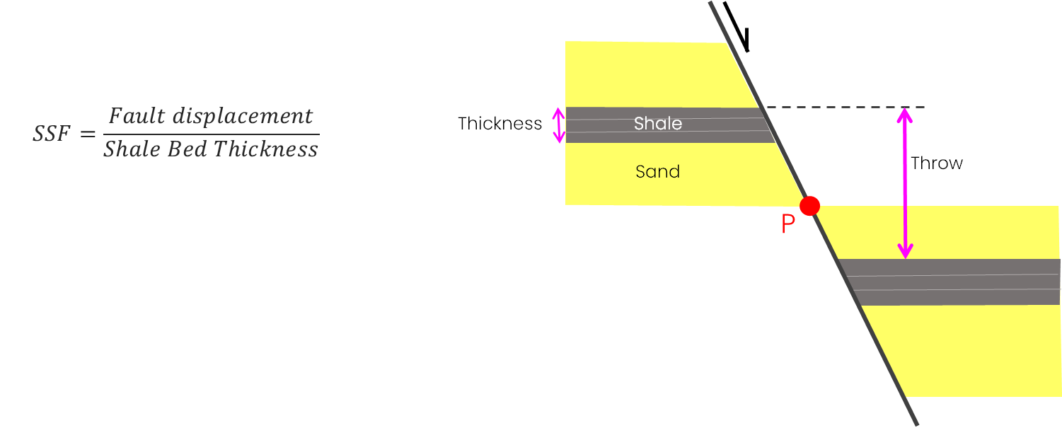
Method 2 - Clay smearing 'Shale Smear Factor' (SSF)

This method is a measure of the amount of intact (continuous, sealing) shale that has been smeared from shale beds into the fault zone. SSF only applies to layers that have been defined as 'shale' in the model by the user-defined Vshale cutoff criterium (optionally combined with a shale layer thickness criterium). In a sequence with multiple shale beds, the minimum SSF value within the slipped sequence (this is the SSF derived from the thickest shale layer in that sequence) is the ultimate shale smear factor at the point of calculation.

SSF is a relatively conservative method, as only defined shale layers are incorporated in the clay content calculation. It produces a constant SSF value at all points between the offset shale layers. By applying a cut-off value, you define the pattern of continuous smears that seal the fault plane and discontinuous smears that are open to flow.

Formula:

where:

Fault displacement = Displacement along the fault (property 'Fault dip displacement') (m)

Shale bed thickness = Thickness of the shale layer after cut-off criterium for Vshale (m)

Calculation example

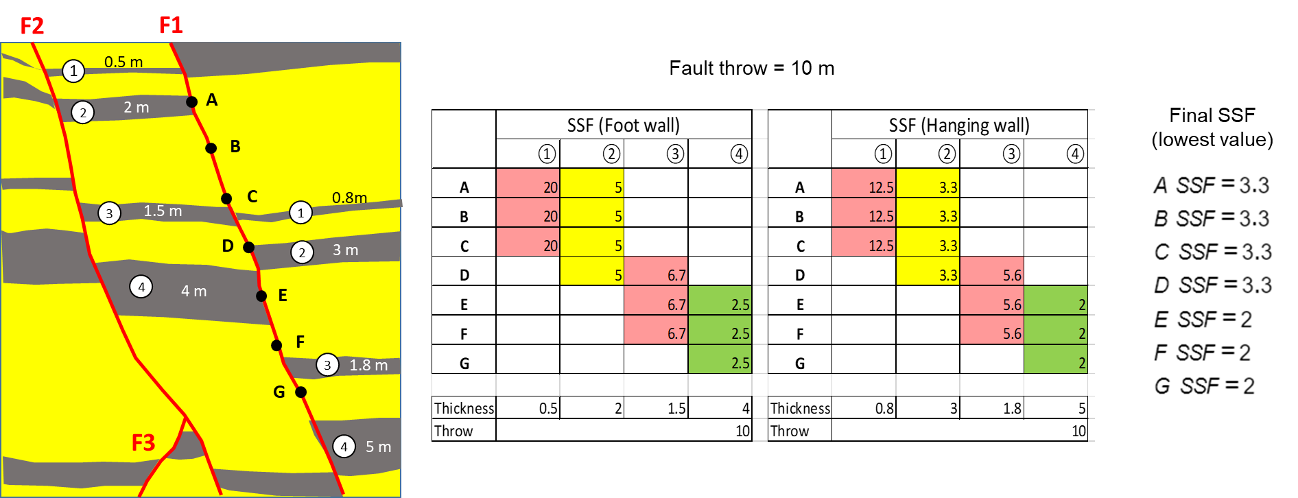
In this example SSF is calculated for points A to G in fault F1 (left image). The gray shale layers are determined by the Vshale cutoff criterium (optionally in combination with a shale layer thickness criterium) on the Fault Clay Content form. Four shale layers are encountered (layer 1, 2, 3 and 4) with varying thickness at both sides of the fault. Per point of calculation (A to G), SSF is calculated for the shale layers of the slipped sequence per footwall and hanging wall side of the fault (left and right table respectively). For example, the slipped sequence of point A consists of two shale layers (layer 1 and 2) with SSF values (using the above formula) in the footwall and hanging wall of 20, 5, 12.5 and 3.3. The SSF assigned to the point of calculation is the lowest SSF value within that range, which means that for point A, SSF is 3.3 (derived from shale layer 2). This calculation forms property SSF smear in the JewelExplorer.

Generated properties:

Three properties are generated:

SSF smear: This property contains the SSF values as explained in the calculation example above, i.e. fault displacement divided by the shale bed thickness, with the final SSF value at point of calculation being the lowest SSF in the slipped sequence (i.e. derived from the thickest shale bed). In the example above, for calculation point A, SSF smear would be 3.3.

When the slipped sequence for a calculation point does not contain shale layer(s) (i.e. the Vsh cutoff criterium and the optional minimum shale layer thickness criterium are not met), the calculation point will be set to undefined in properties SSF smear, SSF categorical and SSF shale bed average.

SSF categorical: Categorical property based on property 'SSF smear' after a 'continuous smear' cutoff value (which you enter on the Fault Clay Content form) has been applied. All calculation points with SSF smear lower than (or equal to) the continuous smear cutoff value are 'continuous' (intact) smears and all calculation points with SSF smear higher than the continuous smear value are 'discontinuous' (disaggregated) smears. In the example above, if continuous smear cutoff value would be set to 3.0, this would mean calculation points A, B, C and D would be 'discontinuous' and calculation points E, F and G would be 'continuous' in property 'SSF categorical'.

The calculation points with SSF values lower than continuous smear cutoff value are called 'continuous' because low SSF values are derived from thick shale source layers, therefore the shale smearing in the fault zone at these locations is considered continuous and unbroken at that particular fault displacement.

SSF shale bed average: Vsh value of the shale layer with the lowest SSF value (derived from the thickest shale bed) in the slipped sequence at point of calculation. This follows the same principle as the calculation of SSF smear, but with the SSF value being replaced with the Vshale value of the respective shale bed. The Vshale value is weighted for grid cell thickness of all grid cells in that shale bed. In the example above, 'SSF shale bed average' for calculation point A is the Vshale value of shale bed 2.

Method 3 - 'Clay mixing, Clay smearing' (SGR - SSF combination)

In this method the results from methods 'Clay mixing' and 'Clay smearing' are combined by means of assigning alternative clay content values for the 'continuous' and 'discontinuous' categories of property 'SSF categorical' (see 'Method 2 SSF', property 'SSF categorical'). For the 'discontinuous' category you can choose from three types of clay content, all SGR-based and generated with 'Method 1 SGR'. To assign clay values to the 'continuous' calculation points, you can choose from three other options (see below). 'SGR - SSF combination' outcomes range between 0 and 1.

Discontinuous

Choose one of the following options to assign clay content values to the 'discontinuous' calculation points in property 'SSF categorical':

Undefined calculation points in property 'SSF categorical' (areas defined as no-smear or discontinuous smear) will receive the value of the selected SGR property.

Average Average SGR of the slipped sequence at the point of calculation (see 'Method 1 SGR', property 'SGR average').

Hanging wall Hanging wall SGR of the slipped sequence at the point of calculation (see 'Method 1 SGR', property 'SGR hanging wall').

Footwall Footwall SGR of the slipped sequence at the point of calculation (see 'Method 1 SGR', property 'SGR footwall').

Continuous

Choose one of the following options to assign clay content values (seal or strong flow baffle) to the 'continuous' calculation points in property 'SSF categorical':

Use constant A constant Vshale value which you can enter on the form.

Use Vshale cutoff value The Vsh cutoff value as applied to 'Method 2 SSF' (option on the form in the Settings section of 'Method 2').

Use average value from shale bed Vsh value of the shale layer with the lowest SSF value (i.e. the thickest shale layer) in the slipped sequence at point of calculation. This is the same principle as which is used to calculate SSF, but with the SSF value now being replaced with the Vshale value of the respective shale layer. The Vshale value is weighted for grid cell thickness of all grid cells in that shale layer (see 'Method 2 SSF', property 'SSF continuous clay').

Generated properties:

One property is generated:

SGR - SSF combination: This property contains the combined results from Method 1 SGR and Method 2 SSF. In essence it is the 'SSF categorical' property with the categorical values overwritten with equivalent clay content values derived from the choices that you make on the form. Clay content values range between 0 and 1.

Methods after:

Yielding, G., Freeman, B., Needham, D.T., 1997. Quantitative fault seal prediction. American Association of Petroleum Geologists, Bulletin 81, 897-917. https://doi.org/10.1306/522B498D-1727-11D7-8645000102C1865D.

Lindsay, N.G., Murphy, F.C., Walsh, J.J., and Watterson, J., 1993. Outcrop studies of shale smear on fault surfaces. S. Flint and I. Bryant, eds., The geological modelling of hydrocarbon reservoirs and outcrop analogues: International Association of Sedimentologists Special Publication 15, p. 113-123.