The model strip
The Model strip contains the functionality to build reservoir models. After preparing your input data using the prepare strip, you will typically work through the Model strip from left to right. If you have faults, you start off with building a fault model, then you continue with creating a structural model, a 3D grid, property model, etc., up to volumetric calculations and reporting. Within each of the model sub-strips (for example Faults, 3D Structure, Fluids, etc), you will typically follow the workflow, located at the left-hand side of the sub-strip, while at the same time having access to various tools located towards the right of each sub-strip.
If faults are identified in your data, you first need to create a fault model. The Faults item is therefore the first item on the model strip. Fault surfaces to be included in the fault model are selected from either the Seismic Interpretation or the Surface Set folder, created during the data preparation step of the modeling workflow. When faults are identified in your well data, they are stored as fault markers in your Marker Set. You can create multiple fault models, each with its own combination of faults. The faults used in the fault model will be re-triangulated to a regular mesh with rearranged nodes and triangles. This facilitates better clean-up of branch lines (referred to as fault-fault intersections).
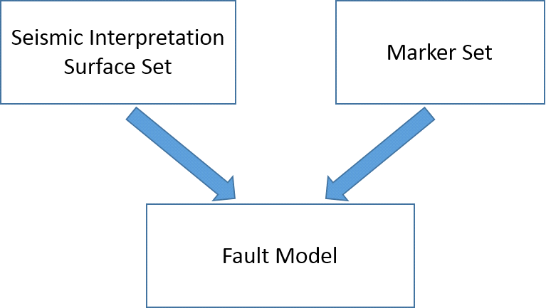
Flow diagram showing how fault surfaces and fault markers interact with the fault model click to enlarge
Fault-fault intersections occur where one fault is truncated by another. Given the typical resolution of a seismic survey, such a situation may be apparent where one fault crosses another without showing an offset (requiring a retraction) or where two faults are very close together and should be connected (requiring an extension). The tools to perform these actions are provided under the Faults item of the model strip. In the Fault Modeling workflow, fault markers (interpreted on the wells) can be matched with the fault surfaces.
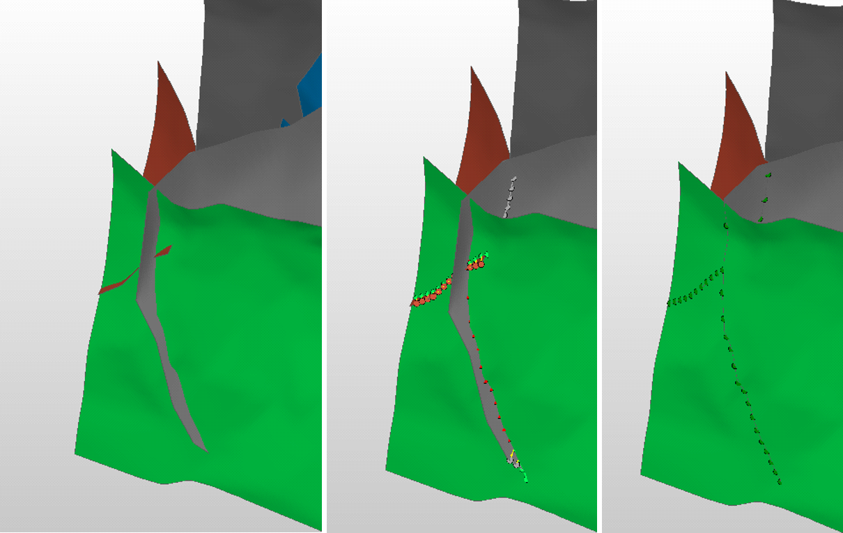
An example of fault retraction click to enlarge
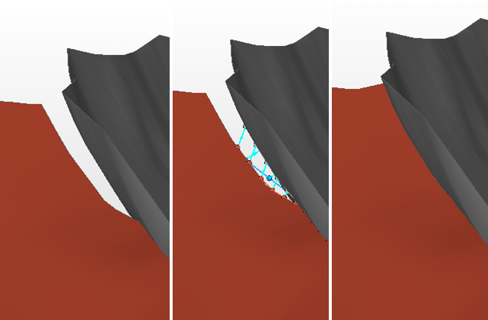
An example of fault extension click to enlarge
Creating a 3D structural model
A fault model and a stratigraphic model combine to create a 3D structural model. Because the stratigraphic model can be created from both seismically-derived horizons and well markers, a fault model, a stratigraphic model and the well markers are required inputs to the Structural Modeling workflow. Under the 3D Structure item of the model strip, tools are provided to clean up fault-horizon intersections (called fault cutoff lines).
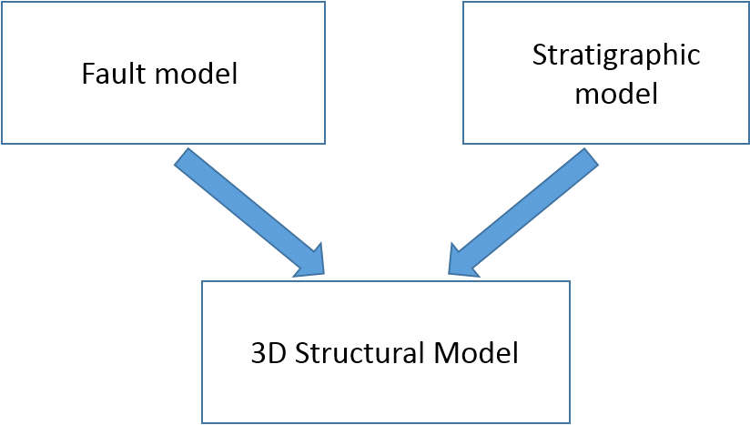
Flow diagram showing how the fault model and stratigraphic model interact with the 3D structural model click to enlarge
As the stratigraphic model can have multiple (hierarchical) levels (see The stratigraphic model) you can choose up to what detail to build the structural model by selecting a level. The image below is a stratigraphic model, containing three stratigraphic levels; it shows zone boundaries based on surfaces and their associated well markers [S,M] (red arrows), and well markers only [M]. You can choose to first build the structural model up to Level 2 and perform QC steps such as editing fault cutoff lines, before creating the full structural model up to Level 3, which includes surfaces based on well markers only.
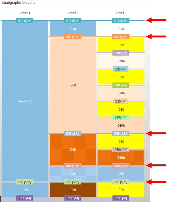
Example of a stratigraphic model in JewelSuite Subsurface Modeling containing three stratigraphic levels. The underlying data to the zone boundaries is either a surface, indicated with an [S] or a marker, indicated with [M]. The red arrows emphasize the zone boundaries based on surfaces [S], which are generally placed on a higher stratigraphic level (Level 2 in this example) than zone boundaries based on markers [M] only (Level 3 in this example). For details, see The stratigraphic model click to enlarge
Horizons interpreted on seismic data may show artifacts near faults as the seismic resolution may not be very clear at these locations. In order to create clean fault cutoff lines, tools are available to clean up horizon areas around the faults. The application will not delete the data in this user-defined area, but make data points inactive. It creates a property on the horizon that is fault model dependent. This allows you to use multiple fault models on one set of horizons, each with its own clean-up distance.
In building the 3D structural model, JewelSuite Subsurface Modeling creates surfaces for all faults of the selected fault model and all the horizons and markers of the selected stratigraphic level. Subsequently, fault cutoff lines can be calculated and visualized (see image below).
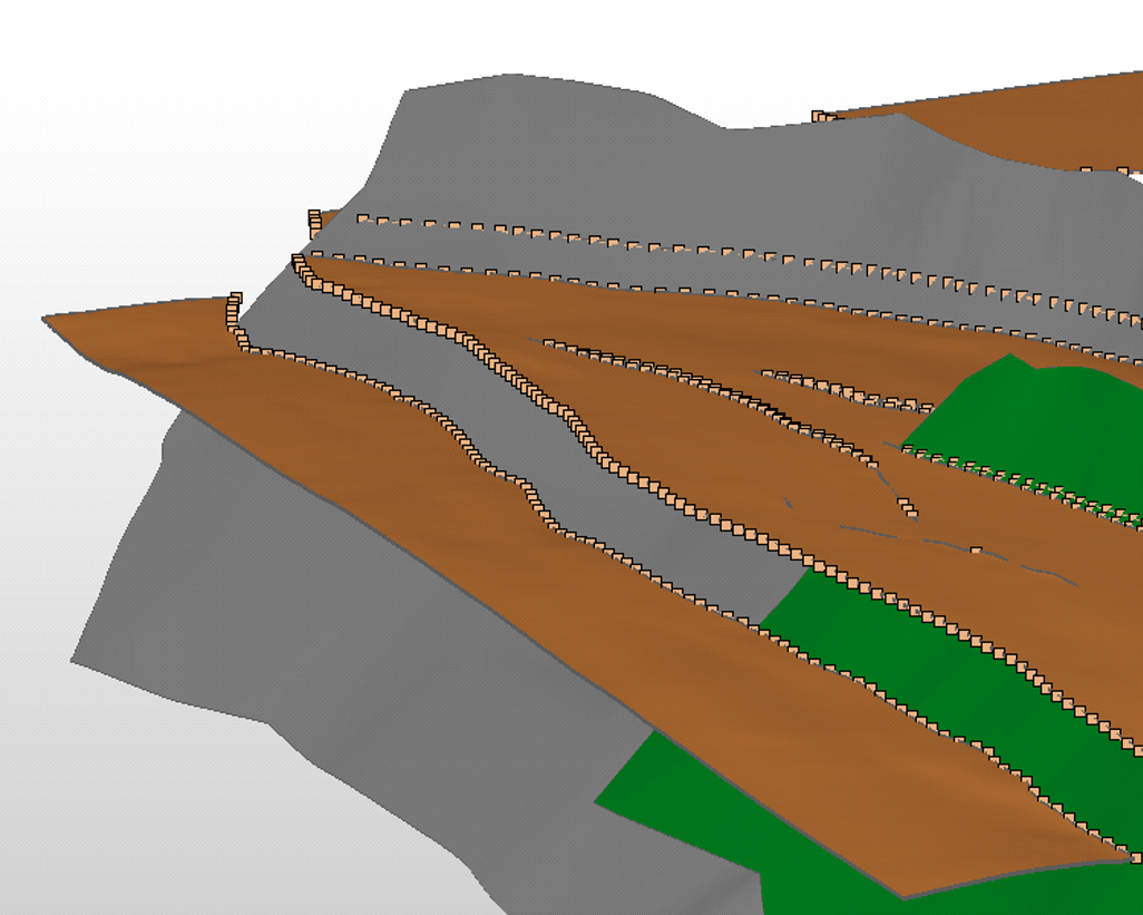
Example of fault cutoff lines, highlighted by nodes, which can be edited with the available tools on the Faults sub-strip click to enlarge
Fault cutoff lines
Fault cutoff lines can be edited by moving the visualized nodes of the footwall and/or hanging wall up or down the fault planes. Once a satisfactory result is obtained, you can recreate the structural model by honoring all edits. The result is a 3D structural model with a fully triangulated, cleaned-up set of horizons and faults.
The 3D grid is the geocellular JewelGrid, based on the structural model which is further subdivided into smaller layers called k-layers. With the 3D Gridding workflow, available under the 3D Grid item of the model strip, you can create a 3D grid zonation; the further subdivision of the structural model zonation into k-layers destined for property modeling and/or reservoir simulation. The image below shows an example for a 3D grid zonation, schematically visualized in a dedicated view (called the 3D Grid Zonation View). In the example, the k-layers are defined in the yellow reservoir zones.
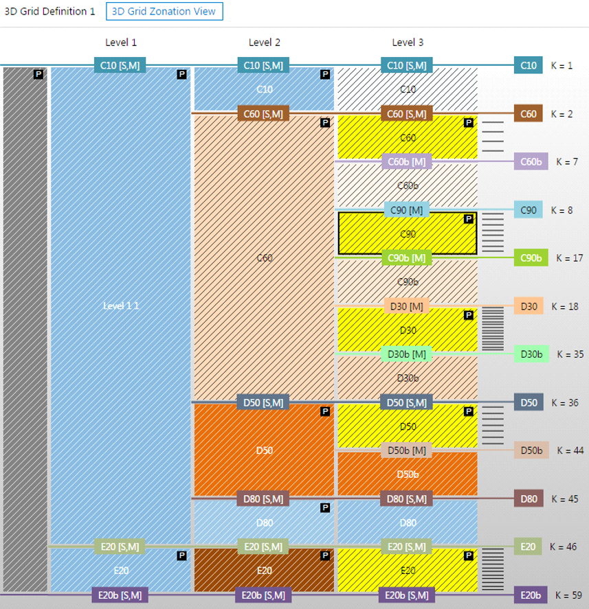
An example of a 3D grid zonation, schematically presented in the dedicated '3D Grid Zonation View'. The yellow reservoir zones are subdivided into k-layers, indicated at the right side of the image click to enlarge
The last step before the grid is generated is the area definition within which the final grid will be created. In this step you define the lateral cell size and the orientation of the final grid.
Adding properties
After creating your 3D grid, you will want to populate the cells with properties for volumetrics calculations and possibly reservoir simulation. A property model is a representation of the distribution of facies and petrophysical properties, scaled up to the resolution of a 3D grid.
After you have upscaled your data, you can create a property model based on upscaled well log data using the model > Facies strip or the model > Rock Properties strip, depending on whether you are working with discrete or continous properties. On the same strips, a set of tools is provided to allow you to fine-tune your model results, or to perform mapping or statistical data analysis.
You can also add properties using tools under the Tools button in the Workspace section at the right side of the strip. With the Property Calculator, you can create and update properties for seismic volumes, grids, tri-meshes and well logs, and with the graphical editing tools you can update grid properties directly by ‘painting’ property values on the grid in a 3D View.
Fluid and saturation models
Accurately determining the initial fluid distribution in a reservoir is vital for volumetrics and dynamic simulation, but generally involves data and workflows that are spread across various subsurface disciplines, such as geology, petrophysics and reservoir engineering. With the fluid model, you combine all the available data and iteratively define (different scenarios of) the initial fluid distribution in the form of 3D compartments and fluid levels.
While the fluid model allows you to predict the fluids in the field using hydrostatic equilibrium and compartment boundaries (surfaces), it is also important to take into account the rock properties and hence predict saturations across the reservoir. Combining the fluid model with a saturation model based on rock-dependent properties and petrophysical analysis, you can then move on to volumetrics and simulation.