Example - Modeling facies with MPS and 3D trend property
In JewelSuite you can create a 3D trend property, a combination of lateral and vertical trends, on the model grid. In the example below, a lateral trend is extracted from the geological concept, while the vertical trend is derived from well log data across the field. Later you can combine both the trends and use it to guide the MPS modeling.
Modeling 3D trend property
In the example below, you build a 3D trend property for a turbidite fan environment on a 3D grid.
Modeling lateral trend
- Create a new 3D grid and create the trend properties on this 3D grid. In this example, create an Easy 3D grid (Model > 3D Grid > Grid Tools > Create Easy Grid) with dimensions of 10000 m x 10000 m x 200 m.
- On the Create Easy Grid form, create a new grid and enter the grid name.
- Create a new area with the dimensions 10000 m x 10000 m x 200 m. Click OK to create the 3D grid.
- Create two new polyline sets using the Editing Tools (Workspace > Tools). Click on the icon
 to add polyline sets, and from the Property Inspector pane change the surface type for both polyline sets to Line. Rename one of the polylines as ‘Source’ and the other one as ‘Spine’. You can use one of the polyline sets as a source to control the energy change and the other polyline as a spine to control the trend pattern.
 - Using the Polyline Set Tools, draw polylines for both the source and spine on the 3D grid (see image below for reference).
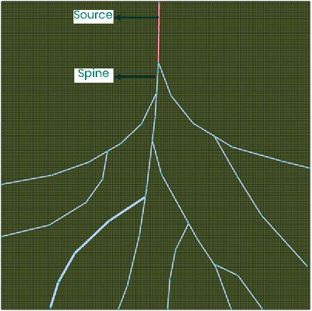

Polyline sets created for source and spine using editing tool. click to enlarge
- Create two new ‘distance from object’ properties. Create two properties for source as well as spine, using the property calculator.
- Open the Property Calculator and at the top of the Property Calculator form, make sure the Target Object is set to your Easy Grid.
- In the Target Property section, create a new property and set the Property Type to 'Distance'.
- Use the Distance... function from the Functions group. On the Distance from object dialog that opens, select the object type to Polyline Set and select Vertical projection (horizontal plane) and click OK.
- The expression is filled in the Expression field. Click OK at the base of the Property Calculator form.
- The result is automatically shown as a property of your Easy Grid in the 3D View. Refer to the images in the first row in the figure below.
- In the next step using the property calculator, reverse normalize the distance values for both the distance from object properties, and generate property type ratio with values from 0 to 1, so the values decreases away from the polyline.
- Start with the first property, for example the distance from object property 'Source'. Open the Property Calculator and at the top, make sure the Target Object is set to your Easy Grid.
- In the Target Property section, select Create New, give the property a name (for example 'Source Trend'), and select Property Type 'Ratio'.
- In the Expression field, enter the expression as given under the left image in the first row in the figure below (make sure the name of the distance to object property (created under step 4) is correctly used in the expression). You do not have to type the full expression, but can select the distance from object property from the Properties and Variables section on the Property Calculator form. Click Apply at the base of the Property Calculator form to create the reversed distance to object property.
- Repeat the above steps for the second distance to object property ('Spine'), and use the expression as given under the right image in the first row in the figure below.
The low energy limits used for this example are arbitrary and will depend on the depositional setting and 3D gird size.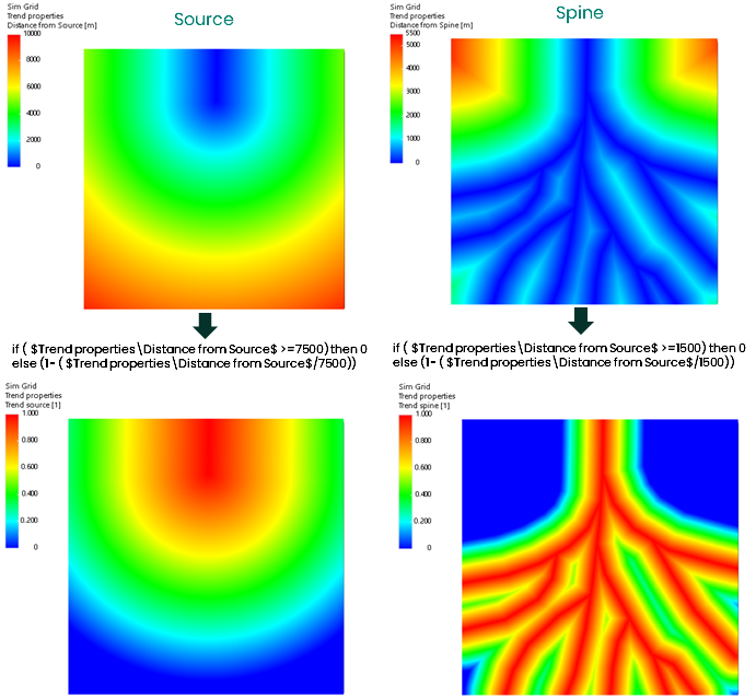

Images in the first row are shows the distance from the polylines (source and spine). Using property calculator and reverse normalization, bottom row shows the resulting trends for source and spine. click to enlarge
- In the last step, combine both the trends (source and spine) to generate the final lateral trend.
- Open the Property Calculator and make sure the Target Object is set to the Easy Grid. Create a new property with the property type ‘Ratio’ and name it ‘Lateral Trend’.
- In the Expression field, multiply both the reversed distance to object properties that were created in the previous step. Click Apply to create the final lateral trend property. Refer to the image below.
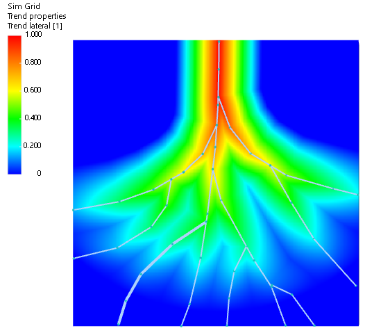
Combination of source and spine trends resulting in the final lateral trend. click to enlarge
Modeling vertical trend
There are several petrophysical methods to create a vertical trend property based on well log data. For this example, you will use a single well log data with VShale log and inverse distance method to populate the upscaled log into the entire grid. The available input data and methods to populate the upscaled properties in your 3D grid may vary depending on several factors like depositional environment, extent of field, well log data, etc.
- Create a new rock property model of the type VShale (Model > Rock Properties > Create Model). On the form, select the 3D grid that was used to create the lateral property and select the entire grid volume definition.
- In the next step, on the Assign Method form select the inverse distance method (IDW) and click OK.
- Click OK to skip the transform & trends form and move to the Control Method form. For the vertical trend, use the calculation type as 2D (layer by layer) and select a power value from the drop down list. Click OK to move to the Run Model form.
- Check the box to select Entire grid VOI and run the model by clicking OK. The resulting vertical trend property is located under the Rock Properties folder of your 3D grid. Refer to the image below for the result generated in this example.
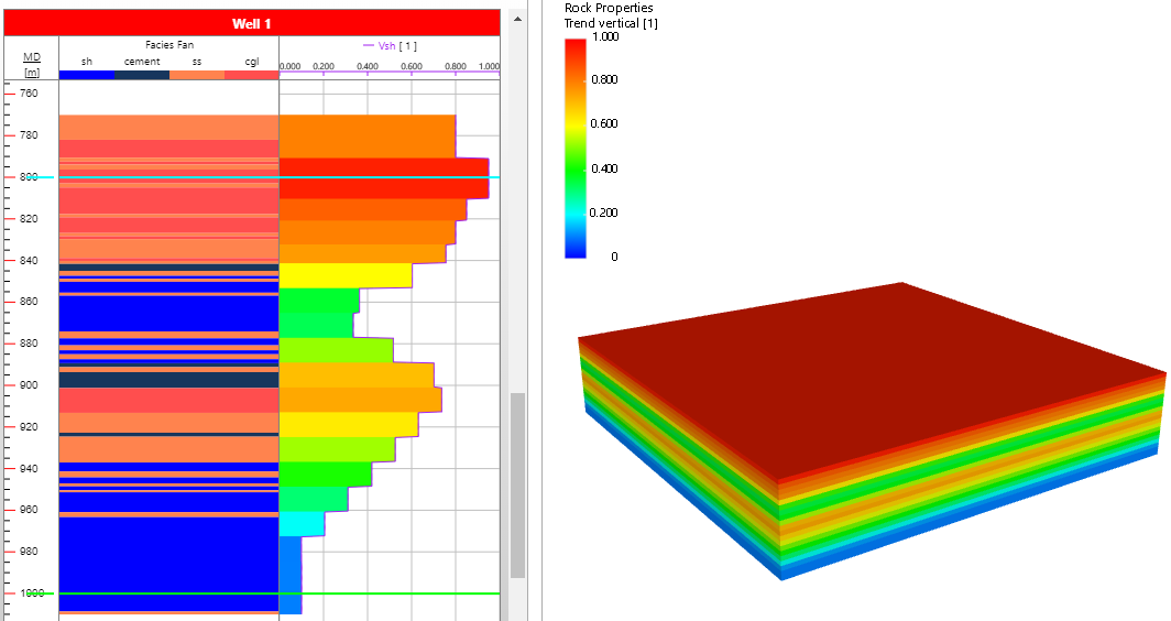

Vertical trend property created using Vsh well log. click to enlarge
3D Trend
Use the property calculator to combine the lateral and vertical trend properties.
- To do this, open Property Calculator and select the 3D grid, that contains both the lateral and vertical trend properties, as the Target Object.
- Create a new property with the Property Type ‘Ratio’ and name the property, for example ‘3D trend property’.
- In the Expression field, multiply the lateral and vertical trend properties and click Apply to generate the 3D trend property.
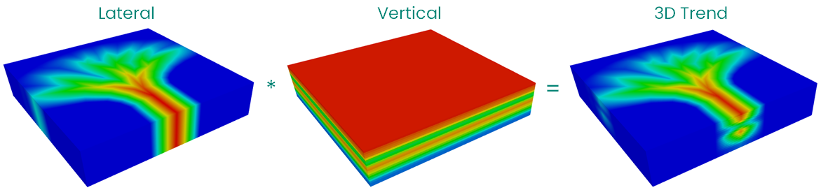
3D trend property created using Property calculator. click to enlarge
MPS Modeling
MPS method like other statistical method requires a stationary condition. However, in geologic reality the trend occurs on a different scale, and to handle this non-stationary condition IMPALA (the MPS technology used in JewelSuite) has the capability to use non-stationary training image together with its trend.
In order to create a facies model (in this example, a turbidite fan environment), use the 3D trend property created in the previous step along with the trend property in the training image (TI). Use the JewelSuite TI Library or Create a training image using the editing tools.
Create trend property on TI
- To create a trend property on a TI, training image is required. In this example, we use a training image from the TI library.
- Depending on the dimensions of the TI grid (in this case 60 x 120 x 1) and direction of deposition, create a trend property that scales from 0 to 1 using the property calculator. See the resulting trend property in the image below.
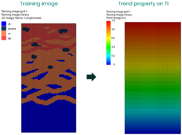
Resulting trend property using training image from TI library. click to enlarge
Building the facies model
- Create a new upscaled facies property for your 3D grid, using the property calculator. Use the context menu of the facies property from JewelExplorer to create 4 classes of facies - shale, cement, sand and conglomerate.
- Create a new facies model (Model > Facies > Facies Modeling > Create Model). In the Assign Data section, select the your 3D grid, the new facies property as the upscaled property, and entire grid as volume definition. Click OK to open the Assign Method form.
- Select MPS from the drop down as the modeling method. Click OK to open the Assign TI form. In the Assign Training Image section, select the training image grid from the drop down and the training image property imported from the TI library. Click OK to apply the settings.
- On the deposition patterns tab of the Trends & Proportions form, check the box adjacent to Depositional Pattern Trend 1. Make sure the training image grid is selected and select the Trend Property in Training Image from the drop down list. This is the trend property on the training image created in the workflow above.
- Select the 3D trend property for Trend Property in VOI from the drop down list. Adjust the TI facies pattern reproduction value with the slider. The higher the weight factor, the more dominant the trend becomes in the facies model.
- On the Rotation tab, check the ‘Rotation’ checkbox to activate the settings. Select the appropriate option that applies to your facies model. In this example, the azimuth of the trend property from depositional trend is used.
- Click OK to save the settings and open the Control Method form. Select Random option under the Simulation Path and click OK.
- On the Run Model form, select entire grid as the VOI. Enter a simulation seed base value or roll the dice to randomly generate a value. You can also create multiple realizations of the facies model by entering a value more than 1. Click OK to run the model. The new facies model is stored under the Facies folder of the 3D grid properties. The resulting facies model is shown in the image below.
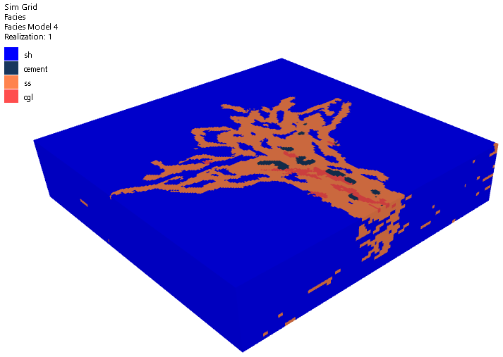
Facies model generated using the MPS method and 3D trend property. click to enlarge