Normal Score
The GSLib algorithms used for geostatistical modeling and simulation expect data to represent a standard normal distribution. A standard normal distribution is a special case of the normal distribution, where the normal, random variable has a mean of 0, and a standard deviation of 1. If a data distribution is skewed and significantly diverts from a standard normal distribution, you must transform the data to create the required distribution. The Normal Score data transformation forces the data to a normal score distribution using a cumulative density curve to rank data and match it to ranks in a normal distribution.
Guidelines
Be careful using the upscaled property to define the target distribution if the input data are limited. The resulting target distribution might include unrepresentative sampling artifacts that will be reproduced in the histogram of the final output. In such cases it is often better to use a user-defined normal distribution or a reference property instead.
The Normal Score transform is not necessary for Kriging or IDW and it is usually best to leave it out. The 'Upscaled property', which is selected by default in the 'Distribution' drop-down list, will introduce discontinuities in the result related to sampling artifacts in the data. If the data are positive a Logarithmic transform is sometimes useful to prevent negative extrapolations in the result. A Shift Scale transform used by itself has no effect on Kriging or IDW.
Be aware that the Normal Score transform does not define the distribution of the property model’s final output if other transforms are present. The data transformations are performed in the specified sequence, with the Normal Score transform last, if present. Afterward, the output of the modeling algorithm is backtransformed using the inverse of the transforms in reverse order. Thus, the Normal Score transform defines the target distribution of an intermediate property prior to application of the other reverse transforms in the sequence.
Normal Score Target Distribution
Distribution There are four options to define the target distribution: (1) Upscaled property, (2) Property with reference distribution, (3) User-defined normal distribution, and (4) Distribution model. The first two options use empirical target distributions, the third and fourth options use distribution models.
- Upscaled property (or 'Property to be transformed' on the '3D Property Preparation' form) is the default selection for the distribution to be targeted on backtransformation. If this property has only a limited number of samples, you should consider to go for any of the other options.
- Property with reference distribution. You can select any continuous property of the same 3D grid to borrow the target distribution. You can also use the property calculator to generate a property with the desired distribution, and select it here. Make sure of the following:
- The values of the modeled, upscaled property need to be within the range of the distribution of the selected property.
- Make sure that if 'Logarithmic' and/or 'Shift Scale' is in your list of transformations the property with reference distribution is dimensionless. Otherwise, the property with reference distribution should have the same property type as the modeled, upscaled data.
- User-defined normal distribution. By providing the mean and standard deviation, you can directly specify the parameters of a truncated Gaussian distribution to be targeted on backtransformation. The values of the upscaled property need to be within the range of the specified distribution.
- Distribution model. For the target distribution, you can use a distribution model. From the Distribution drop-down list select the option 'Distribution model'. When you select a distribution model, its parameters settings are listed as read only fields.
Name Only available when using 'Distribution model'. In the Name field select the name of the model you want to use. To create a distribution model or edit an existing one, click on the edit  icon to open the Distribution Model Tool.
Mean Only editable when using 'User-defined normal distribution'. In other cases it will display the mean of the targeted distribution after backtransformation.
 next to the 'Mean' entry field to open the Uncertainty Parameter dialog. For how to use the controls on the dialog, see The Uncertainty Parameter dialog. For information about parametric uncertainties and how to use them in JewelSuite Subsurface Modeling, see Incorporating uncertainty in static or dynamic modeling.
Standard dev. Only editable when using 'User-defined normal distribution'. In other cases it will display the standard deviation of the targeted distribution after backtransformation
next to the 'Standard dev.' entry field to open the Uncertainty Parameter dialog. For how to use the controls on the dialog, see The Uncertainty Parameter dialog. For information about parametric uncertainties and how to use them in JewelSuite Subsurface Modeling, see Incorporating uncertainty in static or dynamic modeling.
Lower bound / Upper bound (when target distribution is 'Upscaled property' or 'Property with reference distribution'):
Stochastic modeling will generate more values than the input data, extending further into the tails of the distribution. When the target distribution is defined by the Upscaled property it is necessary to specify the target distribution tails beyond the data range. In JewelSuite this is done by specifying lower and upper bounds that are assigned probability densities of zero. The lower bound must be smaller than the smallest data value, and the upper bound must be larger than the largest value. Cumulative probabilities are linearly interpolated for intermediate values. You can specify the lower and upper bounds as percentages or absolute values.
The target distribution may also be specified by a Property with reference distribution. A reference property can have much more data than the upscaled property, in which case extrapolating the tails of the distribution is less of an issue. Nevertheless, it is possible for stochastic simulation to generate values beyond the range of the upscaled data or the reference property so specification of upper and lower bounds is still necessary. The lower bound should be smaller than the smallest upscaled value and the smallest reference property value. The upper bound should be larger than the largest upscaled value and the largest reference property value.
Note that these parameters specify tail extrapolation of a distribution model, not data truncation of input or output. Input truncation can be added as a separate transform, if desired, and output truncation can be controlled in the Control Method workflow step.
Lower bound Set a value for the Lower boundary of the target distribution.
- Absolute Enter the Lower boundary value as an absolute value.
- Relative Specify the Lower boundary value as a percentage of the input data range below the minimum value of the input data. Example: input data range is 1 – 10 and the Relative percentage is set at 10%. The Lower boundary of the target distribution: 1 - (0.1*9) = 0.1.
Upper bound Set a value for the Upper boundary of the target distribution.
- Absolute Enter the Upper boundary as an absolute value.
- Relative Enter the Upper boundary as a percentage of the input data range above the maximum value of the input data. Example: input data range is 1 – 10 and the Relative percentage is set at 10%. The Upper boundary of the target distribution is: 10 + (0.1*9) = 10.9.
Min truncation / Max truncation (when target distribution is 'User defined normal distribution'):
The Min and Max truncation parameters control the limits of a truncated Gaussian distribution model. That is, the tails of the distribution beyond these limits are truncated by setting the probability density to zero, and the interior is normalized so that the total cumulative probability is one. The minimum must be smaller than the smallest data value and the maximum must be larger than the largest value.
To approximate a non-truncated model, you set the minimum and maximum truncation values far enough away from the mean where the untruncated probability density is very small. To approximate a non-truncated Gaussian model, three or four standard deviations away from the mean is usually adequate.
Note that these parameters specify tail truncation of a distribution model, not data truncation of input or output. Input truncation can be added as a separate transform, if desired, and output truncation can be controlled in the Control Method workflow step.
Background to Normal Score transform
The images in the table below illustrate the behavior of the Normal Score transform when used in SGS. These are simplified examples with no other transforms, a variogram with a short range and a sill of one, and no secondary data in the conditioning step. The first row of the table shows the 'Upscaled property' option, the second row the 'Property with reference distribution' option, and the third row the 'User-defined normal distribution' option (selection options from the 'Distribution' drop-down list on the Transform & Trends form when 'Normal Score' is selected under 'Transformations').
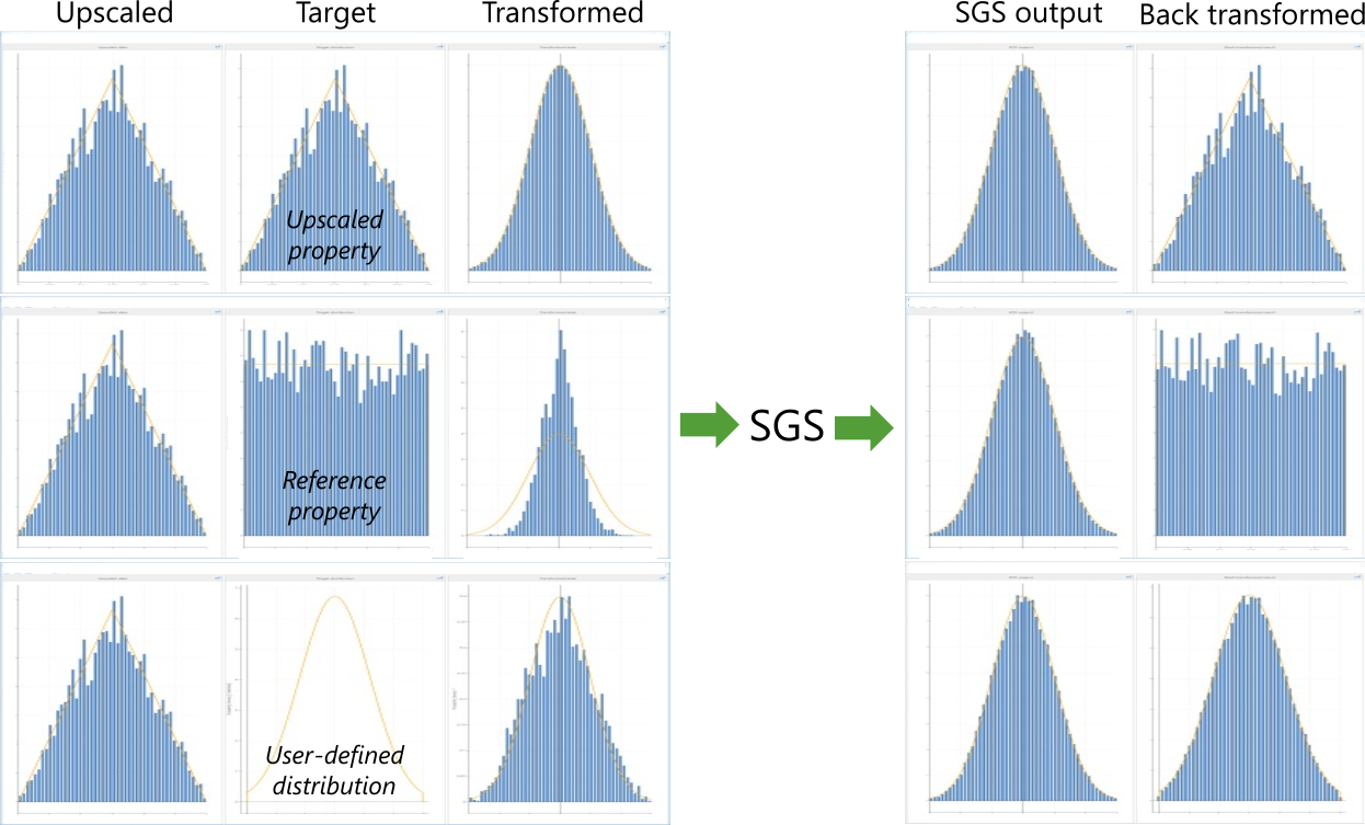
Overview of the effect of the target distribution on the backtransformed data. click to enlarge
The first column shows a histogram of the upscaled data randomly sampled from a triangular distribution, the same for each example. The second column shows the target distribution: the same as the upscaled data for the first example, randomly sampled data from a uniform distribution for the second example, and a truncated Gaussian model for the last example.
The third column shows the result of the Normal Score transform. In the first example the data have become perfectly Standard Normal. For the second and third examples they are not perfectly Gaussian, but that is not actually required for SGS. The fourth column shows that the raw output from SGS is always Standard Normal for these simplified cases, regardless of the input data histogram.
The last column shows the final backtransformed result that approximately reproduces the target distribution in each case. Note that the sampling artifacts of the target distributions are reproduced in the final results of the first and second examples, but the sampling artifacts of the upscaled data are removed in the last example (user-defined distribution).