Reservoir simulation using a JewelGrid
From a lateral perspective, a JewelGrid is composed of a 100% rectangular pattern. This results in a regular lateral IJ-grid, with vertical 'stacks'. Each stack (more accurately stack set, see below) is fully determined by its i- and j-value. On the other hand, layers are fully determined by their k-value. The vertical grid boundaries of the grid cells are determined by k-layer definition, faults, intrusions, and unconformities (the latter three called 'discontinuity surfaces' or 'discontinuities'). This allows for a highly accurate representation of these geological phenomena, even within the dimensions of an IJ-stack.
The cross-section in the figure below shows the effect of layering and a reverse fault.
Note that in the following description both 'layer' and 'k-layer' are used, meaning the same feature, namely a layer consisting of a single cell in the vertical direction
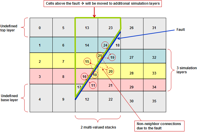
Effect of layering and a reverse fault click to enlarge
Although each k-layer has a unique k-value, the fault results in that a layer may have two, or even more, grid cells with an IJ-stack. For example, the yellow layer, with say k-value 2 (top undefined layer has k=0), has two grid cells namely cell 15 and 10, in the third IJ-stack from the left. Let’s assume this IJ-stack has i=3, and j=5. Hence, both cells 15 and 10 have i=3, j=5, and k=2. These grid cells are called multiple-IJK cells. Most reservoir simulators cannot handle this, and, in order to correctly model a JewelGrid in a reservoir simulator, a grid is built that the simulators can handle. This grid is called the simulation grid.
Note that apart from grid cells adjacent to faults, intrusions, or unconformities, the JewelGrid results in almost rectangular grid cells, with only the dipping of the layers resulting in not 100% perfect orthogonally. This unique feature of JewelGrid cells results in a very accurate finite difference definition in the simulator resulting in most correct modeling of flow (convection), diffusion, and heat conduction.
Before going into detail, a few concepts should be explained.
- A stack is all the cells with the same i- and j-value above (top stack), below (bottom stack), or in between discontinuities. This means that all cells within a stack always have a unique k-value.
- A stack set is composed of all stacks with the same i- and j-value. A stack set is defined by its i- and j-value.
- A multi-valued stack set is a stack set that has two or more stacks.
- Multiple-IJK cells are cells that have the same i-, j-, and k-value.
- A schematic grid is a schematic representation of a simulation grid.
Creating a simulation grid from a JewelGrid
To correctly model a JewelGrid in a reservoir simulator, a grid is built that simulators can handle. In the following we will call that grid the simulation grid.
In the simulation grid, multiple-IJK cells are taken care of by adding additional k-layers (as compared to number layers in the JewelGrid layers) to the simulation grid and storing multiple-IJK cells in these layers. Non-neighbor connections (also called special connections) are created to connect these multiple-IJK cells to their actual neighbors in the JewelGrid. Subsequently, transmissibilities for both neighbor and non-neighbor connections are calculated.
Although porosity, net-to-gross and permeabilities to the simulator are automatically specified, and the simulator subsequently calculates the pore volume and transmissibilities, these simulator calculated values are overwritten with its own calculated values.
The creation of a simulation grid from a JewelGrid will be explained by using a simple example of a grid with three layers and a reverse fault. The figure above shows a 2D-slice of this example grid. Two IJ-stack sets have been used to accurately represent the fault. Along this fault, non-neighbor connections have been defined.
To explain the creation of the simulation grid, take a look at the following example description. In this example case the creation of the simulation grid entails adding extra grid k-layers for the simulation. These layers are used to store blocks of cells which are situated directly above faults, unconformities, or intrusions. For example, the cells above the reverse fault in the figure (marked by a green boundary) are moved to additional layers.
The resulting simulation grid is illustrated in the next figure. Notice that the number of layers has doubled and that the cells above the reverse fault have been moved to the new layers. The empty space created above the fault and in the new layers is filled with void cells. These void cells will be ignored by the simulator. Additional non-neighbor connections have also been defined between the moved cell block and its previous direct neighbors. You may notice that this way is not the most efficient way of storing the multiple-IJK cells, but this is the simplest way to explain the basics of the method.
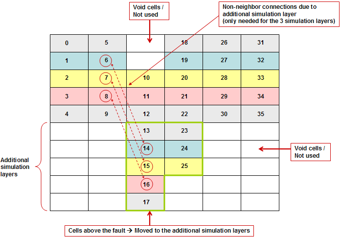
Resulting simulation grid with additional layers to store multiple-IJK cells click to enlarge
All defined non-neighbor connections will be specified in the input file(s) to the simulator (see below).
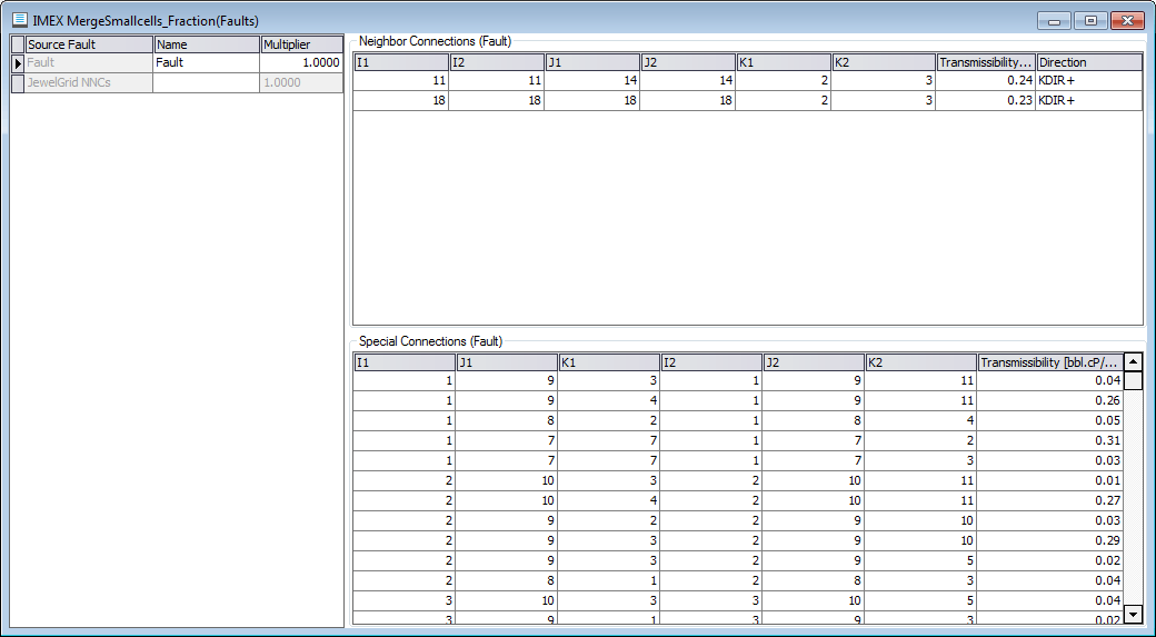
Non-neighbor connections are specified in the input file click to enlarge
Apart from just blindly reallocating multiple-IJK cells, functionality is also provided to reduce the number of multiple-IJK cells by merging them with neighbor cells. For example, cell 25 could be merged into cell 15 and cell 10 into 20, thereby reducing the number of additional cells in the grid by two. During these operations the total pore volume is maintained and the connections are property reallocated. For example, if cell 10 is merged into cell 20, the transmissibility of connection between cells 15 and 10 is added to the transmissibility of connection between cells 15 and 20.
In most situations all multiple-IJK cells are able to be merged and so no additional layers are created in the simulation grid.
When do we really need to do simulation grid preparation? Simulation grid preparation is only necessary in case of multiple-IJK cells, i.e., in case two or more cells have the same i-, j- and k-value.
How the resulting simulation grid looks like depends on the simulation grid creation settings (Reservoir Description form, step Simulation grid creation settings) and the values of the key properties, i.e., porosity, permeability and net-to-gross.
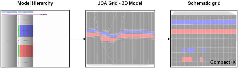
By default, the created simulation grid remains invisible. If you click Create schematic grid in the 'Diagnostics' step of the Reservoir Description form, a schematic grid similar to that shown in the figure above is created and can be analyzed in a 3D view, for example.
Note that the schematic grid is, as the name suggests, just a schematic representation of the simulation grid. For example, in the schematic grid all cells have uniform thickness and the added layers are vertically positioned below the actual layers. In the simulation grid, the cells in the added layers will have the same cell center depth as the corresponding cell in the JewelGrid. For example, in the figures above, while cells 6 and 14 have different depths in the schematic grid, in the simulation grid the have similar depth.
Each time you build a new input dataset a check occurs which indicates whether the simulation grid has to be recalculated. This is required when simulation grid creation settings have changed and/or when one or more of the key properties has changed. Also, each time you (implicitly) ask for a new simulation grid creation, a check is performed to see whether a simulation grid created with the same parameters and properties already exists. If the latter is the case, the existing simulation grid is used. This may, for example, be the case if you have done you history matching and are evaluating alternative development scenarios.
When a simulation grid is created, a property folder is created in the JewelExplorer under the grid linked to the simulation case. The name of the folder is the name of the case for which the simulation grid was created plus 'SimGrid'. This folder contains the grid properties of the simulation grid. Examples of properties created are, the simulation grid i-, j-, and k-values (named SimI, SimJ, and SimK), and in case cells are merged, a property named 'Merged Cells' which indicates which cells have been merged, or not.
Simulation grid creation options
Four options to create a simulation grid from a JewelGrid are provided, namely:
- Include impenetrable layers
- Merge multiple-IJK cells
- Merge small cells
- Merge pinch-out cells
The settings shown above are the default settings.
The effect simulation grid creation options have on the creation of the simulation grid will be discussed in detail below.
This basic method is not the default method (see above), but it is the simplest to explain and a good starting point.
Cells in different stack sets have by definition different i- and/or j- value and hence can never be multiple-IJK cells. Hence, we only need to consider cells within a stack set.
A stack set with only a single stack will by definition not have any multiple-IJK cells, as within a stack all cells have different k-value.
Hence, only multi-valued stack sets will contain multiple-IJK cells and need to be dealt with to create a proper simulation grid.
The basic method discussed first has the following options set:
- Include impenetrable layers
- Merge multiple-IJK cells
- Merge small cells
- Merge pinch-out cells
The basic method uses the following logic:
- A grid is created that has the same lateral dimensions as the source JewelGrid, i.e., same number of cells in i- and j-direction, and has the double plus one number of k-layers. (An extra layer in between the main (original) layers and the additional layers is created to enable connection of aquifers.)
- For every multi-valued stack set, the stack with the most cells is placed in the main layers of the simulation grid.
- Missing cells in these main layers are eventually taken from the other stacks, starting with the cells with largest volumes (the reason for this is minimization of the number of non-neighbor connections).
- All remaining cells from other stacks are placed in one set of additional simulation layers.
- In case two or more stacks need to be placed in the set of additional simulation layers, cells will be located automatically in the set of additional simulation layers, as efficiently as possible.
- Non-neighbor connections, fault surfaces, and transmissibilities are used to properly connect all cells in the simulation grid.
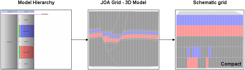
Example of the basic simulation grid preparation method. Only one set of additional simulation layers is created in the simulation (schematic) grid to hold the additional cells due to faulting. Also, the impenetrable layers are present in the simulation (schematic) grid click to enlarge
Generally, there is no reason to include impermeable layers in your simulation model as this is just adding to the size of the simulation, irrespective of how efficient a simulator treats inactive cells. Hence you will not generally include impermeable layers and will disable 'Include impenetrable layers':
- Include impenetrable layers
- Merge multiple-IJK cells
- Merge small cells
- Merge pinch-out cells
Example of the basic simulation grid preparation method with option 'Include impenetrable layers' disabled; impenetrable layers are NOT present anymore in the simulation (schematic) grid click to enlarge
The advantage is that the simulation grid has fewer layers. As the excluded layers contained only inactive cells:
- This default method will give exactly the same simulation results as the basic method.
- Excluding impenetrable layers will have a minor positive effect on running time of the simulator.
- Input and output files for the simulator will be smaller.
For these reasons excluding impenetrable layers is default.
Simulation grid creation – merge multiple-IJK cells
We will discuss here the basic method but now with also the Merge multiple-IJK cells option enabled:
- Include impenetrable layers
- Merge multiple-IJK cells
- Merge small cells
- Merge pinch-out cells
As the name suggests, the application tries to merge multiple-IJK cells with neighboring cells, thereby reducing the number of multiple-IJK cells and hence reducing the need to reallocate cells in the simulation grid.
The following logic to merge cells is used:
- Within each stack set, cells with the same k-value are compared and the cell with the largest volume will be placed in the main layers. All other cells with the same k-value will be merged with neighbor cells on the main simulation grid layer and on the same side of the fault, unconformity, or intrusion. These neighbor cells will be in neighboring stack sets.
- If it there is no neighbor cell in the same layer and on the same side of the fault, unconformity, or intrusion, a neighbor cell in an adjacent layer will be chosen.
- In most cases all multiple-IJK cells can be merged and hence no additional layers are created in the simulation grid.
- However, in the rare situation that a neighbor cell to merge into is not available, additional layers will be created to accommodate the multiple-IJK cells. Such a rare situation may for example arise at the wedge where two faults intersect.
- The connections, both neighbor and non-neighbor, of the merged cell are added to the connections of the neighboring cell into which it is merged.
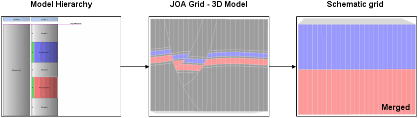
Example of the use of the 'Merge multiple-IJK cells' option. In the example above, additional layers are not created in the simulation grid as all multiple-IJK cells could be merged into neighbor cells click to enlarge
The main advantage of using the merge multiple-IJK cells option is that the resulting simulation grid is much smaller than with the basic option as in most cases no additional k-layers are created in the simulation grid and hence a simulation grid of less than half the number of grid blocks as compared to the basic method is created. Also, in most cases, the number of non-neighbor connections will be much less.
The local coarsening due to cell merging influences the simulation results. This effect is larger when the fault (or unconformity, or intrusion) density is high, that is, when there are laterally few cells in between faults. It is good simulation practice to check the effect on simulation results of simplifications, if possible. The same applies here, and you should make sure the difference between results with and without cell merging is acceptable by running a simulation with and without merging.
The Merge small cells option can be enabled independently of the other options.
- Include impenetrable layers
- Merge multiple-IJK cells
- Merge small cells
- Merge pinch-out cells
Any simulator has the option to exclude small cells, i.e., make them inactive. The criterion to make cells inactive is minimum pore volume (e.g., PVCUTOFF keyword in CMG simulators and MINPV and MINPVV in the ECLIPSE™ simulator). The default pore volume cut-off value is zero, that is, only cells with zero pore volume are made inactive. Cells made inactive this way do not contribute to the total volume of the system, and are treated as a barrier.
The simulator just makes these blocks inactive and, hence, any pore volume of these cells and possible flow across these cells is set to zero.
Eliminating small cells reduces the number of active cells and eliminates cells that potentially may cause numerical convergence problems, thereby reducing calculation time. The idea is that small cells don’t effect overall volumetrics and flow behavior. If small cells cause convergence problems then they must have significant flow and, hence, eliminating them affects flow in the simulation.
The 'Merge small cells' option does not just make small cells inactive, but merges small cells with neighboring cells in the same layer and reallocates the connections of the merged cell to the cell in which it is merged. Hence, both total volume of the system is maintained and no barriers are created.
As a result, the 'Merge small cells' option has the benefits of the inactivation of small cells by the simulator but not the disadvantages of it.
The 'Merge small cells' uses 'Fraction of average cell volume in same layer' as cut-off criterion. This is better than the generic minimum pore volume criterion used by simulators as the user may have small cells (e.g., small layers) in parts of the model to accurate model flow behavior (e.g., small layers at top of reservoir to model gas overrunning), while having large layers in parts of the reservoir where accurate simulation is less important (e.g., aquifer layers). The criterion used by the application ensures that small cells in areas where small cells are required are not inactivated.
The 'Merge pinch-out cells' option can be enabled independently of the other options.
- Include impenetrable layers
- Merge multiple-IJK cells
- Merge small cells
- Merge pinch-out cells
Any simulator has the option to exclude these pinch-out cells. The difference with the minimum pore volume option and the pinch-out option is that in the latter criterion the simulator will automatically generate non-neighbor connections between the active cells on either vertical side of the pinched-out layer(s), allowing fluid to flow across it. Generally, the layer or layers of inactive cells are deemed to be pinched-out if their overall cell thickness is less than the specified threshold value.
The option works similarly in the application, also using cell thickness as the criterion. The difference between the 'Merge small cells' option and the 'Merge pinch-out cells' option is that the former uses (relative) cell volume as a criterion while the latter the cell thickness.
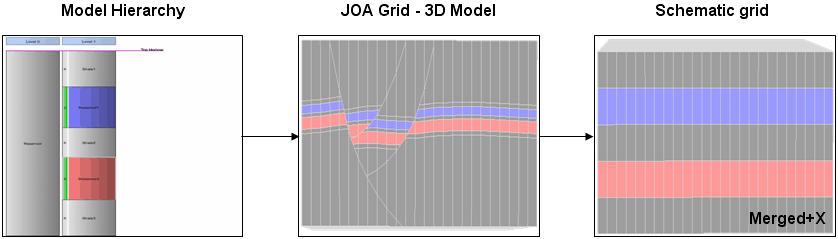
The four options may be used in any combination. For example in the figure below the effect of combining 'Exclude impenetrable layers' and 'Merge multiple-IJK cells' is shown.
Example of the use of 'Exclude impenetrable layers' and 'Merge multiple-IJK cells', resulting in a simulation grid with only two layers click to enlarge
The effect of the merge options may overlap. For example, a particular cell may be merged because it happens to be a multiple-IJK and/or a small cell and/or a pinch-out cell. In case of selecting multiple merge options:
- Identifies and merges pinch-out cells
- Identifies and merges multiple-IJK cells
- Identifies and merges (remaining) small cells