The JewelGrid in the modeling workflow
Construction of the JewelGrid
The required inputs for the JewelGrid are surfaces defined by 2D grids, polyline sets, tri-meshes, point sets or well marker sets. Different representations can be combined to represent one geological event (e.g. a horizon, fault, etc.). The process of grid construction is stepwise (see image). Of these steps, the first four steps are performed with the structural modeling workflow, resulting in a structural model with internal stratigraphic zonation (here, the JewelGrid is used as explained below, but 'under the hood'). Step 4 takes place in the Structural Modeling workflow (resulting in the 3D Structural Model), Step five takes place in the 3D Gridding workflow (resulting in a 3D grid with internal k-layering).
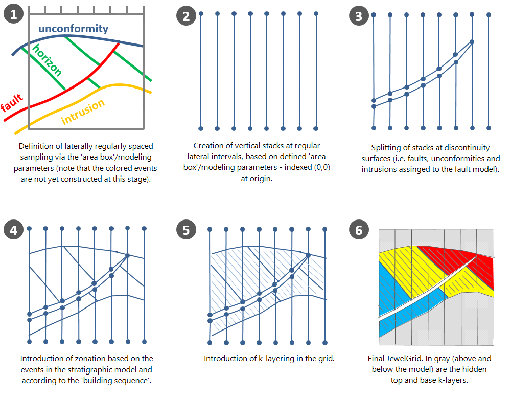
Step 1 First the area is defined, specifying the lateral grid cell dimensions and azimuthal rotation.
Step 2 At these regularly distributed locations, pillars (vertical lines) and stacks (vertical elements in between 4 pillars) are defined. Each of these stacks has an I and J index attached to it. These indices are 0, 0 at the origin of the 3D grid and increase in when moving away from the origin.
Step 3 At discontinuities defined in the fault model (i.e. faults and unconformities/intrusions assigned to the fault model), the vertical stacks are split into two stacks.
Step 4 Stratigraphic horizons are inserted (according to the 'building sequence'), respecting the discontinuities and resulting in a structural model with internal (stratigraphic) zonation.
Step 5 K-layers are inserted within each of the (stratigraphic) zones.
Step 6 The resultant JewelGrid has a top and base defined by the unconformity and intrusion respectively. However the nodes of the stacks are defined in Step 1. Therefore, an overburden and underburden k-layer is also created (which is normally hidden although can be visualized). The depth index for the JewelGrid starts with k=0 so that the first visible layer has k=1.
The JewelGrid and property modeling
Conversion of the JewelGrid to a flat orthogonal simulation grid or box ('simbox') required by most property modeling algorithms is a relatively straightforward task. Only vertical translations are required owing to the vertical stacksets of the JewelGrid. The figure shows how the JewelGrid deals with an example of simple linear interpolation across a fault. In this example the two cells cut by the fault have a common IJK index and are represented by the same cell in the simulation box. The value in this cell is then shared by cells on re-splitting during translation back to the structure grid.
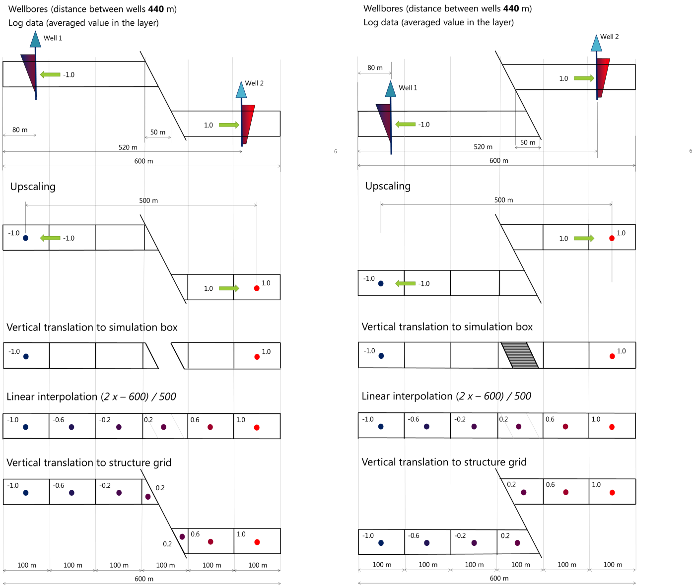
Sequential steps demonstrating property interpolation in the JewelGrid simulation box for a normal faulted (left) and reverse faulted layer (right) click to enlarge
Where a well passes through a faulted cell the original upscaled value is preserved in the simulation box. If the well passes through both hanging wall and footwall cells (for example, a vertical well passing through a reverse fault), either the average value of the two cells, or the value of the hanging wall cell (this depends on the fault throw) is used by the property modeling interpolation algorithm and the original cell value is pasted back in during the reverse translation back to the JewelGrid.
The lack of lateral shifts in the simulation box transformation is a clear advantage over the traditional pillar grids as the lateral dimensions of geobodies (for example, channels) are preserved.
The JewelGrid and flow simulation
As in the property modeling simulation box, simulator decks also require a vertical translation of cells within a stack set. The property modeling simulation box assumes that all cells were laterally connected during deposition and restores them accordingly. The simulation grid requires a slightly different approach in order to preserve the correct present day flow pathways across faults.
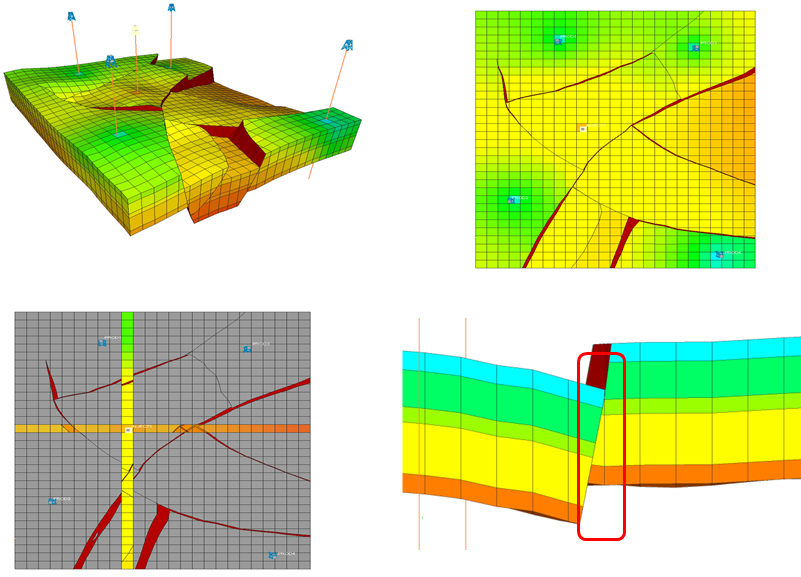
The views in the top row show that most of the JewelGrid is orthogonal in the lateral direction; the vertical faces of a cell are perpendicular. A stackset can be identified with an I and J index, which is visualized as the crossing of the east and north slice in the third view. More than one stack can be present in a stackset as can be seen in the last view where part of a slice with five layers is shown. This brings us to an important characteristic of the JewelGrid. There are IJK indices that denote more than one cell. click to enlarge
A part of simulation preparation is the determination of the mapping of IJK indices between the JewelGrid and the simulation grid. When no faults are present, the mapping is simple and the number of IJK indices in the JewelGrid is equal to the number of IJK indices in the simulation grid. When faults appear, this is no longer the case. In the JewelGrid it is possible to have more than one cell with the same IJK index. More precisely a column identified by an IJ index can have more cells with the same K index. This situation occurs near faults as shown above . Most often two (near a fault) or three (near truncating faults) cells share the same IJK index.
The process of conversion of a JewelGrid and associated property arrays to a simulation grid is as follows:
- Model Upscaling - Upscaling of the JewelGrid and associated property arrays to simulation-scale, if required. The results are visualized in JewelSuite Subsurface Modeling.
- Transmissibility Calculation - The permeability and shape of two neighboring cells are in general not the same. For this reason, the transmissibility between cells is obtained through serial addition of the two cell contributions. Here the cell contribution is the transmissibilities between the cell center and the center of the face common to the two cells. Transmissibility is calculated for all cell connections.
- IJK Mapping and Merging - Where multiple cells share an IJK index, as explained above, they are mapped into an orthogonal grid definition and cells with multiple IJK indices mapped into deeper k-layers (see below).
- Transmissibility property mapping and calculation of Non-Neighbor Connections - Transmissibility is not an intrinsic cell property but a property. Transmissibility between adjacent cells is calculated and transferred to the modified cells in the simulation grid by mapping into cells as a property. If neighbor cells in the JewelGrid are not neighbors in the simulation deck, the connection is achieved using non-neighbor connections. A non-neighbor connection contains the IJK indices of the cell to connect and the transmissibility between them. In addition to transmissibility the volumes and depth of each cell are preserved and specified to the simulator.
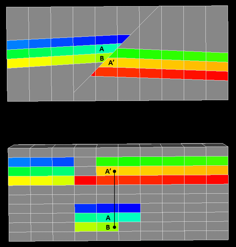
Example of the re-mapping of multiple cells with identical IJK indices from the JewelGrid (upper image) to the simulation grid (lower image). In this example cells A and A' have an identical IJK index and cell A is re-mapped. Cells A' and B are juxtaposed in the JewelGrid requiring a non-neighbor connection (indicated with a black line) in the simulation grid. The example is taken from the JewelSuite pre-processor click to enlarge
Simulator performance improvements can optionally be realized by merging small cells and pinch out cells or, in an extreme case, all multiple index cells. In the merging process, the transmissibilities are updated.
Summary
In summary, the JewelGrid is a near orthogonal grid with faulted cells which combines geometrical flexibility and can be created easily without extensive user interaction. The known limitations of pillar grids in geometry handling are serious blockers when integration purposes require models to be laterally and vertically comprehensive. The JewelGrid and UVT Grid both overcome the topological constraint of the pillar geometry.