Performing well correction

When depth and thickness uncertainty is applied, all impacted surfaces will obtain a shift relative to their original position in the structural model, also at the well locations where they were potentially well-matched. With the Well Correction form (model > 3D Structure > Well Correction) you can choose to correct uncertainty-induced depth shifting at well locations, as well data can be key control points for your structural model. Well correction brings back the surface to its pre-shift position at the well locations. In other words, it brings back the surface to its original position in the structural model, which might or might not correspond to the marker, depending on whether the surface was well matched.

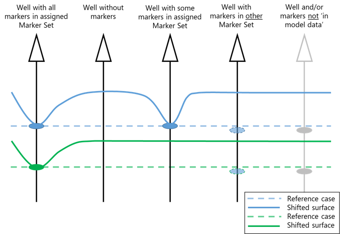
When a surface is selected for well correction on the form, it will get corrected in those wells which have a marker for that surface in the Marker Set assigned to the Structural Model. click to enlarge

On the form, you can select the surfaces to be included in the well correction. Available for selection are all surfaces in the 'seismic' and 'sub-seismic' tables of the Define Uncertainty form (including surfaces bounding the intervals), up to and including the selected 'Stratigraphic level' (at the top of that form), except 'fixed' seismic surfaces. It then depends on the presence of a marker for the selected surface, whether or not the surface will be well corrected. More specifically, well correction for a surface in a particular well only takes place when a corresponding marker exists for that well in the Marker Set assigned to the Structural Model (given that the well and marker are both 'active', i.e. not 'switched off' via the 'Use for modeling' or 'In model data' options, see 'Use for modeling' in Marker Table). This is schematically displayed in the diagram above.

Well correction of a surface can impact the depth shift (around the well) of surfaces that are hierarchically of lower order (see How depth shifts are calculated). This is due to the fact that well correction takes place immediately after depth shift calculation of a surface and before the depth shift calculation of the next (lower order) surface.

Note that when well correction takes place in a certain well for a particular surface, the correction will take place at all surface intersections in that well and irrespective of the marker location(s). In other words, when a surface-well intersection exists multiple times in a well (typical for horizontal wells), the surface will be shifted to its pre-shift position at all these intersections, see image below.

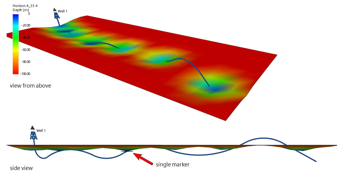
When a surface gets corrected to its pre-shift position, correction takes place at all intersections in that well, irrespective of the marker position(s). click to enlarge

Given that the depth shift at the well locations has to be zero, but honored at certain distance from each wellbore, two interpolation techniques are provided (IDW and Kriging). Based on these interpolation techniques, a smooth transition is created from the well location (zero shift) to the depth shifted areas. The extent of this transition area around the wellbore is determined by the 'radius of influence' which you can enter on the form. These well correction settings will be applied when running a volumetric study with the study strip.

To perform well correction

At the top of the form, select the Structural Model for which you want to perform the well correction.

In the Well Correction table, select the surface for which you want to apply well correction.

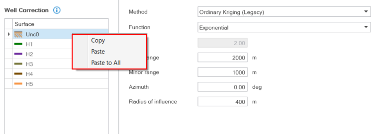
Right-mouse click on a surface to copy-paste the settings on the form to other surfaces. click to enlarge

Method Per surface, specify the well correction (note that once you're done, you can copy-paste your settings to other surfaces):

None

When you select 'None' (default setting), no well based depth shift correction will be applied to the selected surface.

Inverse Distance Weighting (IDW)

This method uses the inverse distance-weighted algorithm to interpolate the data.

Power - Enter the weight value for the algorithm.

See further below for descriptions of Radius of influence.

Ordinary Kriging (Legacy)

This type of Ordinary Kriging does not make use of the industry standard Kriging library and is performance optimized.

Function - Choose a variogram type to control how the variogram model is auto-fitted to the data:

Spherical
Exponential
Exponential Power - Set the value in the Power entry field underneath, which sets the lateral extension of the Kriging.
Gaussian

A default value of 0.0001 is used for the nugget effect of the variogram model.

Major range - Specify the distance at which the values become independent (the variogram reaches its plateau). The distance is measured in the direction with the greatest spatial continuity.

Minor range - Specify the distance at which the values become independent (the variogram reaches its plateau). The distance is measured in the direction with the least spatial continuity and is orthogonal to the major direction.

When your data does not have anisotropy, enter the same value for both the Major range and Minor range.

Azimuth (GN) - Enter the azimuth (angle with Northing direction) of the axis corresponding with the major range.

Radius of influence - Outside of your 'Radius of influence', the depth shift map is not impacted by the well correction multiplier.

Do not forget to repeat the above steps for each surface to which you want to apply well correction. You can use the copy-paste option by right-mouse clicking on a surface in the table.

Click Apply to save the settings and keep the form open or OK to save the settings and close the form. These settings will be applied to each depth map realization that you create with the Volumetrics Study workflow of the study strip.